
Introduction
ACT General Intelligence is adaptive test that gives an accurate measurement of a person’s general thinking level in a short space of time. ACT General Intelligence consists of three sub-tests: digit sets, figure sets and verbal analogies, which are used to determine numerical analytical capacity, abstract analytical ability and verbal analytical ability respectively. Taken together, these three sub-tests are used to calculate a general intelligence score, known as the g score. ACT General Intelligence was primarily developed for selection purposes.
This guidebook follows the structure of the Cotan (2009) assessment system with regard to the quality of tests:
- Basic principles of test construction
- Testmaterial
- Guide for test users
- Norms
- Reliability
- Construct validity
- Criteria validity
1. Basic principles of test construction
This chapter takes a closer look at the concept of intelligence and examines a number of theories. It also looks at the use of intelligence tests to measure intelligence. The second part of this chapter contains a comprehensive overview of the development of ACT General Intelligence and item response theory, the mathematical model used.
1.1. Theories on intelligence
This section discusses the most relevant theories on the concept of intelligence. Only psychometric theories will be discussed here. There are also other theories that approach intelligence from a different angle (for example, cognitive psychological theories and neurological-biological theories). Their main focus is on describing intelligence as opposed to measuring it. As ACT General Intelligence falls within the psychometric tradition, we have chosen to only deal with this approach. If you are interested, you can find more information on theories that take a different perspective in, for example, Gardner (2011).
Psychometric theories are all based on the differential, also known as the psychometric or correlational school of psychology. The most important point within this vision on psychology is the study and measurement of individual differences with regard to psychological characteristics (Walsh et al., 1990).
Galton’s General Mental Ability
The first person to study the concept of intelligence in the scientific sense was Galton (1883), who formulated a theory of general mental ability at the end of the 19th century. This theory is based on the idea that as all information reaches us via our senses, intellect is the sum of all simple separate aspects of sensory functioning. According to Galton, intelligence stems from the speed and precision of our sensory responses to environmental stimuli. Cattell (1890) developed a range of tests to measure these separate parts of the human intellect, such as tests to measure the ability to ascertain differences in measurements, colour and weight. He called these tests mental tests. There turned out to be scarcely any correlation between the tests and therefore they did not appear to measure any overall general mental ability. Furthermore, these tests were rather impractical, due to the number of different tests required to measure the construct and the numerous repetitions needed to obtain a reliable score. By the start of the 21st century, this view of intelligence had become obsolete (Walsh et al., 1990; Janda, 1998).
Binet-Simon
Around the same time as Galton and Cattell, Alfred Binet and Theophile Simon were developing a clearly different theory on human intelligence. Their goal was to develop a test that could distinguish mentally disabled children from children who were developing normally. Binet and Simon thought that intelligence was part of the “higher mental processes” (such as judgement and reasoning). They also stated that the capacity to implement these higher mental processes should increase with age. A child’s Binet-Simon score was interpreted as his or her mental level or mental age. This test attracted a great deal of attention and was reworked by Lewis Terman in 1916, and by others later on to produce what is now known as the Stanford-Binet test, which is used to determine the “Intelligence Quotient” or IQ.
Spearman’s Two-Factor Theory of Intelligence
Charles Spearman (1923) examined Galton and Cattell’s tests using Factor Analysis, a technique that he had developed. In contrast to other researchers, he concluded that many of these tests showed a positive mutual correlation. From this, he drew the conclusion that a general mental ability, as defined by Galton, actually existed and named it general intelligence or g – a conclusion that is still considered valid today. He also stated that test scores were caused by two components: the g factor and factors specific to the test in question, which he called “s”. This theory is known as Spearman’s Two-Factor Theory of Intelligence (Spearman, 1923). Intelligence as g can be defined as follows:
“Intelligence is not what we know at a specific moment, but how well we can reason, solve problems, think in abstract terms and manipulate information flexibly and efficiently, particularly when the stimulus material is new to a certain extent” (Walsh et al., 1990).
Thurstone’s Primary Mental Abilities
Spearman’s theory was not generally accepted by his peers. One opponent of the two-factor theory was Leon Thurstone (1938). Thurstone stated that the overlap between different intelligence tests was not caused by the g factor, but by the fact that the same skills were required to solve a specific test. Thurstone thought that intellectual functioning could best be described as a collection of independent skills and used multiple factor analysis to formulate thirteen of these primary mental abilities. To test these abilities he developed a battery of tests, known as Primary Mental Abilities Test (PMA). Thurstone’s theory is, along with that of, for example, Guilford (1964, 1967), an example of a Multiple Factor Theory of Intelligence. Guilford (1977) proposed that human capacities could best be described by a combination of three dimensions: five mental ‘operations’ (cognition, memory, divergent production, convergent production and evaluation), five types of content (visual, auditory, symbolic, semantic and behavioural) and six products (units, classes, relations, systems, transformations and implications). As Guilford hypothesised that the three dimensions were independent of each other, this produced 150 (5x5x6) theoretical independent intelligence components. Guilford (1982) had to conclude, however, that this independence could not be proven empirically as there appeared to be a positive connection between the different specific capacities.
Multiple factor versus hierarchical models
One characteristic of multiple factor theories is that they assume that all factors are equal with regard to importance and generality. Other researchers, however, thought that it was possible to demonstrate a hierarchy in factors using factor analysis, a hierarchical model containing both a general factor and specific factors. What they were actually proposing was a combination of Spearman’s and Thurstone’s models. This perspective on analysing scores in mental tests resulted in the Hierarchical models of the nature of mental abilities. Examples of researchers who developed such models include Vernon (1960) and Burt (1949).
Fluid and crystallized intelligence
Another example of a hierarchical model – and probably one of the most famous – is that of Cattell (1941, 1963, 1971), which he went on to develop further with Horn (Horn & Cattell, 1966, 1967). The Cattell and Horn model divides g into fluid intelligence and crystallized intelligence, a categorisation that has become generally accepted (Kline, 1992). This can be defined as a hierarchical model, as the factors of fluid and crystallized intelligence are found between g and scores in specific tests (e.g. ‘verbal comprehension’). Crystallized intelligence involves the application of acquired skills, knowledge and experience. Culture and education therefore influence crystallized intelligence. Although it is not the same as memory, use of long-term memory is also an important component. Tests that measure crystallized intelligence mostly show what someone has already learned: tests that measure a person’s knowledge of history and geography or their vocabulary are measuring crystallized intelligence. Fluid intelligence, on the other hand, measures a person’s ability to reason logically and to solve new problems in new situations, separate from knowledge that has already been acquired: therefore, fluid intelligence is considered more as a fundamental characteristic with a genetic basis. This is why g is associated more with fluid intelligence than with crystallized intelligence.
Conclusion
As we have seen, there are many different theories on intelligence. There is still no full consensus on what exactly intelligence should be understood as and which psychometric theory provides the best description of reality. In a summary of the psychometric theories on intelligence, Kline (1992) concluded that a middle ground between hierarchical and multiple factor theories can be considered as the most realistic option. The existence of g, or a general intelligence factor can be inferred from the fact that scores for the different sub-tests that make up intelligence tests show a reasonable degree of correlation. However, the extent of this correlation does not exclude the existence of more specific factors. Kline’s (1992) conclusion also forms the basis of ACT General Intelligence.
1.2. Intelligence tests
As we have seen in the previous chapter, a wide range of intelligence tests have been developed over the years, from Cattell’s sensory tests up to the Stanford-Binet test, which is still in use today, albeit in a thoroughly revised fourth edition (Thorndike et al., 1986). There are a number of ways in which to classify intelligence tests.
Classification according to ways of conducting tests
One of these classification systems is whether tests are taken individually or in a group (Walsh et al., 1990). Individual tests are conducted by a specially trained person and taken individually. These tests contain elements that involve the use of all kinds of materials or whereby the time must be recorded. The candidate’s performance must be observed in order to produce a score. The Stanford–Binet is an example of such an individual test. Group tests enable large numbers of people to take the same test at the same time. Naturally, the advantage of this type of testing over individual testing is its cost-effectiveness. There is also more standardisation with regard to conducting the test than in individual testing. The disadvantage of this type of testing is that it takes less account of specific individual factors and therefore provides a less comprehensive description of the subject. One famous example of a group test is the Army Alpha that was developed by Yerkes and his colleagues and introduced in 1917 to quickly assess the capacities of the large numbers of recruits for the First World War. ACT General Intelligence can be categorised as a group test as it is fully standardised and taken via computer. In practice, however, candidates often have to complete tests individually as part of a selection procedure.
Classification according to content
As well as distinguishing tests by the method used to conduct and score them, it is also possible to categorise tests on the basis of their varying content. One can distinguish between verbal tests (language, spoken or written), non-verbal tests (figures, symbols) and performance tests (puzzles, mazes). There are also tests that consist of just one item type: a well-known example of this is the Raven Progressive Matrices (Raven, 1936; Raven, Raven, & Court, 2003). In line with the g theory, it is more usual to combine different tests with different item types (resulting in different ‘scales’) in a test battery. These test batteries often combine tests with verbal items and non-verbal items. Well-known examples of this include the international Wechsler Intelligence Scale for Children (WISC; Wechsler et al., 2003), the Wechsler Adult Intelligence Scale (WAIS; Wechsler, 2008), and in the Netherlands, the Drenth Higher Level Test Theory (Drenth Testtheorie Hoger Niveau (DTHN; Drenth, Van Wieringen & Hoolwerf, 2001)). ACT General Intelligence may also be placed in this category of tests.
Classification according to cultural specificity
Finally, it is possible to distinguish tests according to the cultural specificity of the test content. In culture-load
ed tests, the emphasis is on knowledge and skills taught within a specific culture’s education system. Culture-free items are non-verbal items and performances that are not specific to any particular culture or taught at school (Walsh et al., 1990). ACT General Intelligence tries to make items as culture-free as possible. Regardless of the test or item type, the assumption is that scores indicate a subject’s general thinking abilities and therefore ‘load’ on g – this also applies to ACT General Intelligence.
1.3. Theoretical premises of ACT General Intelligence testing
1.3.1 Measuring objective
ACT General Intelligence was developed for selection purposes: it is a tool to provide insight into a candidate's intellectual abilities in order to help test users make a sound, well-informed choice during selection processes. An important reason for using this form of testing is the fact that g is the most important predictor of job performance (Schmidt & Hunter, 1998) – more important than other possible variables, such as personality (Schmidt & Hunter, 1998). A secondary goal is that differences between people – such as differences between people with a non-migrant background and people with a migrant background – should influence the measurement as little as possible as this will also influence the outcome.
Although ACT General Intelligence was primarily developed for selection purposes, it can also be used for other assessment objectives, such as career-related issues that make it necessary or desirable to assess a person’s cognitive abilities.
1.3.2 Choosing a theoretical model for ACT General Intelligence
Kline’s (1992) conclusion forms the basis of ACT General Intelligence: it assumes a general intelligence factor, known as the g factor, based on the fact that scores for different sub-tests show a correlation, whereby the extent of this correlation does not exclude the existence of more specific factors.
Although there is some agreement on the existence of g, there are still discussions on the best way to model scores in intelligence tests (see Jensen and Weng, 1994 and Gignac, 2016), whereby the models from section 1.1 still form the basic starting point. Jensen and Weng (1994) demonstrated that although many different models are possible, g is generally a better predictor of a wide range of outcomes than scores obtained in separate tests. In other words, no matter how you model g: “Almost any g is a “good” g and is certainly better than no g.” (Jensen and Weng, 1994, p. 231). This is an important reason why the basic premise of ACT General Intelligence is the g factor.
Not only is there no full consensus on which model to use, there is also no full agreement on the exact meaning or interpretation of g. Terms like “mental energy”, “generalised abstract reasoning ability” and “single statistical quantity” have been used to define it (Janda, 1998). We can cautiously state that both Binet’s emphasis on the ability to judge and reason, and Spearman’s principle of learning from relations and correlations form the basis for our current conception of intelligence. We ascribe to the definition formulated by Walsh et al. (1990) and stated on pages 5 and 6.
In conclusion, we can state that Ixly’s ACT General Intelligence model is based on the measuring objective (and Schmidt and Hunter’s results concerning this objective), the conclusions drawn by Kline (1992) and the aforementioned definition formulated by Walsh et al. (1990). This entails that the model used by Ixly consists of a range of tests, each of which measures a different aspect of intelligence, while assuming an overall general intelligence factor, the g factor. The basic premise when developing Ixly’s capacities tests is to apply them primarily to the work situation. As different jobs require different capacities, in practical situations one will want to gain insight into the specific capacities necessary for a particular job by using sub-tests. Sub-tests can be used to chart a specific aspect of intelligence that is relevant in a particular situation. For example, it is important to test the numerical abilities of a person who has applied for a financial job. Verbal capacities are less important for this type of job, but there are other jobs for which they will be much more important. Although these specific insights are important, in practice, a person’s general thinking ability is more likely to be the subject of testing, as this is the most important predictor of performance at work. (Schmidt & Hunter, 1992, 1998, 2004). In short, although the scores for specific tests provide qualitative insight into a person’s general thinking ability, selection decisions must be made primarily on the basis of the g (general intelligence) score. The scores for specific aspects of intelligence will be related to each other as they ensue from a person’s general intelligence (g). The scores for specific aspects or intelligence will be related to each other as they ensue from a person’s general intelligence (g).
1.3.3. Culture-free testing
Background
In recent decades, there has been a great deal of emphasis in the Netherlands on the possible partiality (also known as test bias or item bias) of psychological tests when taken by people from ethnic minorities (people with a native Dutch background versus people with a migrant background). Partiality is at play if test scores have different meanings for certain groups. Partiality is also at play if the relation between the test score and a criterion – such as the relation between intelligence and work performance – differs for certain groups (differential prediction; Van den Berg & Bleichrodt, 2000). Partiality may occur for a number of different reasons, for example, due to differences between groups with regard to language skills, familiarity with the manner of testing or familiarity with specific cultural concepts. For example, two people who do not differ from each other in intelligence could obtain different test scores because one is dyslexic and the other is not.
It is clear that partiality is a problem as it means that test scores are not comparable. Certain groups could be put at a disadvantage if important decisions (such as selecting a candidate for a job) are made on the basis of these scores.
Tools are primarily designed by and for members of a specific culture or society. Cultural distortion may occur if they are then used by a group from a different culture, (Bochhah, Kort & Seddik, 2005). Language problems or disadvantages may increase this distortion (Bleichrodt & Van den Berg, 2000). It is therefore important to guarantee that the test scores of people with a non-migrant background and people with a migrant background are comparable and do not show any cultural distortion. In 1990 the report Toepasbaarheid van psychologische tests bij allochtonen [Applicability of psychological tests on subjects with a migrant background] (Hofstee et al., 1990) concluded that many tests were of little or no use when applied to people with a migrant background because the difference in scores between people with a native Dutch background and people with a migrant background was too large and/or the test did not seem to be measuring the same construct for both groups. Many tests, however, did not contain any information on possible test bias. The report recommended that more research be conducted on test bias among ethnic minorities. Ten years later, new reports were published (Bleichrodt & Van de Vijver, 2001; Van de Vijver, Bochhah, Kort & Seddik, 2001) which concluded that apart from a few exceptions (e.g. the MCT tests; Bleichrodt & Van den Berg, 1997, 2004) the situation had not improved. In 2005, the most widely-used tests in selection procedures were assessed for partiality. This assessment revealed that there were still important differences between tests in this area (Bochhah, Kort & Seddik, 2005). From 2011, a work group from the Dutch Institute of Psychologists (NIP) and Cotan have been placing more emphasis on fairness (being free of test bias) during the assessment of psychological tests and their work has led to the inclusion of a fairness matrix in new test assessments in 2015.
Implementation
Following on from the above, we consider it crucial that personal characteristics that are not relevant for measuring the characteristic (intelligence) do not influence either the test results or how they are interpreted. Therefore, during the development of ACT General Intelligence every effort was made to keep the test culture-free insofar as possible. This basic premise has influenced the choice of sub-tests, item development and language use (for example in the instructions).
With regard to language use, we have tried to use simple words wherever possible. There is more information on this in Chapter 2. When formulating items for Verbal Analogies we tried to use as few difficult words as possible (there is more about this in the Verbal Analogies section), and to avoid using racist, sexist, ethnocentric and androcentric expressions (Hofstee, 1991).
The choice of sub-tests in relation to culture-free testing will be discussed in the next section.
Choice of sub-tests
The two most important principles when choosing sub-tests for general intelligence were culture-free testing and the theoretical basic premise (see section 1.3.2). We therefore chose sub-tests that had shown a low cultural bias and a high loading on the g factor in previous studies (see following sections), which primarily measured fluid intelligence as opposed to crystallized intelligence.
Three adaptive sub-tests have been developed that together form ACT General Intelligence: Digit Sets, Figure Sets and Verbal Analogies. These tests can be used to determine a person’s numerical analytical abilities, abstract analytical abilities and verbal analytical abilities. Together these tests produce a g factor score, which can be referred to as general mental intelligence.
We can generally state that the choice of these three sub-tests builds upon a long tradition of intelligence measurement, a tradition that has repeatedly proven itself. There is a plethora of test batteries to measure intelligence and we know that in almost all of them a distinction can be made between the domains of verbal, numerical and abstract/figurative abilities (see, for example, Guttman’s radex model, 1954, 1969). This distinction is often made in academic research (see, for example Ackerman, Beier, & Boyle, 2002). More specifically, most tests feature sub-tests that are similar to the Digit Sets, Figure Sets and Verbal Analogies contained in ACT General Intelligence (Drenth, Van Wieringen & Hoolwerf, 2001; Wechsler, 2008). Many short forms of more comprehensive test batteries, for example, contain at least one of these tests (Pierson, Kilmer, Rothlisberg, & McIntosh, 2012; Sattler, 2001, 2008). They are therefore quite ‘traditional’ intelligence tests. The specific substantiations of the choice of sub-tests with regard to culture-free testing and the theoretical basic premise of ACT General Intelligence are explained below.
1.3.3.1. Digit Sets
The concept of Digit Sets is already very old (Thurstone, 1938). During a Digit Sets test, candidates are required to recognise a logical pattern in a series of digits: as this involves recognising patterns, logical reasoning and solving new, unfamiliar problems, digit sets tests primarily measure fluid intelligence. However, they also require some calculating abilities and therefore the test also measures crystallized intelligence to some extent. Intelligence tests will almost always be a mixture of both (see, for example, Kaufman & Horn, 1996).
The items are non-verbal: this ensures that the sub-test can also be used for candidates with a deficiency in the Dutch language, who speak Dutch as their second language or are dyslexic. As the test measures fluid intelligence it is reasonably culture-free. Because a candidate’s calculating ability can be influenced by their education (which can be related to cultural background) this sub-test is less culture-free than, for example, the Figure Sets (see next section). Research with the Multicultural Capacities Test (MCT-M, Bleichrodt & Van den Berg, 1997, 2004) has shown that there were no significant differences between people with a native background and second-generation migrants when it came to the digit sets test (Van den Berg & Bleichrodt, 2000). We must note, however, that MCT was specifically designed to prevent cultural differences in test scores.
1.3.3.2. Figure Sets
During a Figure Sets test, candidates are asked to discover a pattern in a series of figures and apply it in a logical manner. This test type, which is often also referred to as a matrix test, was developed in the 1930s (Raven, Raven & Court, 2003). Matrix tests are believed to measure general mental ability (g), as evidenced by their high loading on the g factor (Spearman, 1946).
Figure Sets tests measure fluid intelligence. Fluid intelligence tests are considered as being more culture-free than crystallized intelligence tests, but this type of test is generally considered as being an entirely culture-free test because it uses abstract figures and can keep verbal instructions to a minimum (Bleichrodt & van de Vijver, 2000). The Dutch Institute of Psychologists (NIP) has also concluded that this type of test is suitable and useful for testing members of ethnic minority groups (Bochhah, Kort & Seddik, 2005). These tests are often used in cross-cultural research and are frequently used for candidates with an ethnic minority background.
Although a number of features in Figure Sets items differ from each other, they are the same with regard to a number of important aspects. First of all, as with the Digit Sets, all items are non-verbal. This means that this test is suitable for candidates with a deficiency in the Dutch language, who speak Dutch as their second language or are dyslexic. Secondly, as we have said, it is culture-free. Therefore, the tasks use culture-independent signs and drawings. This means that candidates do not require any knowledge of a particular society in order to answer the items. Therefore the test can be used for candidates from different cultures and backgrounds. Finally, the items’ content is not something that is learnt at school: this is the greatest difference with the Digit Sets sub-test. Digit Sets always contain a calculation component. This is not the case when using Figure Sets. All this means that the Figure Sets sub-test is a fair, culture-free test whose results are less distorted by background variables.
1.3.3.3. Verbal Analogies
As the name suggests, the Verbal Analogies test has a verbal component. Tests for verbal abilities generally show greater cultural differences than non-verbal tests (Van den Berg & Bleichrodt, 2000), occasionally to an alarming extent (sometimes between 1 to 2 standard deviations; Evers & Te Nijenhuis, 1999; Resing, Bleichrodt & Drenth, 1986).
In view of the verbal component, one could quickly come to the conclusion that this test measures crystallized intelligence. However, this is not necessarily true: verbal tests (for example, analogies) can be designed so that they load on fluid intelligence. This is the case if the words used are easy and it can be assumed that everyone is familiar with them (Cattell, 1987; Horn, 1965). The test is then about perceiving more complex relationships and patterns between fundamental elements, something which requires little or no previous knowledge. Verbal Analogies tests that use simple, well-known words can therefore also be considered as a good indication of g (Holyoak & Morrison, 2013; Spearman, 1946). This is in contrast to tests that really measure verbal ability, such as tests that require a candidate to conjugate a verb correctly: this can be seen as a test of crystallized intelligence.
For the reasons set out above, we tried to use easy, well-known words insofar as possible when developing items for the Verbal Analogies test. The complexity of an item must be derived from the complexity of the relationships, not from the words it uses. Despite these efforts, however, there will always be differences in linguistic knowledge and vocabulary that might influence the results. We can therefore expect that out of all three sub-tests, this is the sub-test that will pick up most on crystallized intelligence. Research has shown that verbal analogy tests are not culture-free: candidates with a migrant background often have lower scores for verbal analogy tests than candidates with a non-migrant background (see, for example, Van den Berg & Bleichrodt, 2000). However, these differences are small (Meulders & Vandenberk, 2005). Empirical research with ACT General Intelligence has also shown that the differences in this test are relatively small in comparison to other tests (see Chapter 6).
Conclusion on the choice of sub-tests
Figure Sets are the most culture-free tests within ACT General Intelligence as they do not make any demands of a candidate’s verbal abilities. This cultural element can be taken into consideration when conducting these tests. The three tests can be divided into verbal/non-verbal tests as follows: Figure Sets and Digit Sets tests can be referred to as non-verbal tests, while Verbal Analogies is clearly a verbal test.
1.4. Adaptive Capacities Test (ACT) of General Intelligence
The explicit objective of ACT General Intelligence is to make our test culture-free insofar as possible, something which was not a specific goal of many – mainly older– tests. Another major benefit of ACT General Intelligence is that it is an adaptive test. The benefits of this will be explained in more detail in the rest of this chapter, but we want to emphasise here that an important result of adaptive testing is the extremely short time needed to take the test. Taking approximately 30 to 40 minutes, ACT General Intelligence can give an accurate estimate of a person’s intelligence level within a very short space of time, especially in comparison to other tests.
Adaptive testing
ACT General Intelligence measures intelligence in an adaptive manner: candidates sitting an adaptive test are always set the best (=most informative) item selected for their level on the basis of their previous answers.
More specifically, it works as follows: candidates are first given a question at approximately an average level. Their individual level (referred to hereinafter as theta (θ)) is then determined on the basis of their answer. On the basis of previously set criteria, a new item, one that is most informative for this level will be selected from the large item bank. The new θ will then be determined on the basis of this answer, after which the best item will once more be selected, and so the process continues. The test will stop once θ has been measured with sufficient accuracy and what is known as the stop criterion has been reached.
1.4.1. Benefits of adaptive testing
Adaptive testing has several advantages over more traditional, linear tests.
Testing at the right level
Candidates are always tested at their own level on the basis of previous answers. This means that we do not ask candidates with a low level questions that are too difficult for them or ask candidates with a high level questions that are too easy. The assumption is that candidates will be more motivated to take this test rather than traditional, non-adaptive tests (Linacre, 2000; Mead & Drasgow, 1993; Sands & Waters, 1997; Wainer, 1997; Weiss & Betz, 1973). People with a lower level will be less demotivated or put off by items that are too difficult for them, while people with a higher level will not become bored or careless because items are too easy for them (Wise, 2014). Other studies, however, seem to suggest that adaptive testing can be demotivating because for example, people taking a test are not given any easier items in-between (to ‘catch their breath’/receive confirmation of their abilities) and are unable to skip any questions (Frey, Hartig, Moosbrugger, 2009; Hausler & Sommer, 2008; Ortner, Weisskopf, & Koch, 2013; Tonidandel, Quiñones, & Adams, 2002). This last point, however, is not unique to adaptive tests. Also the fact that in an adaptive test more difficult items are set relatively more quickly, leading to a correct percentage of approximately 50%, could also affect motivation (Colwell, 2013). Clearly stating the test’s adaptive nature in the instructions has an important positive influence on motivation and performance in adaptive tests (Wise, 2014). Therefore we have chosen to explain the adaptive procedure (albeit in a simple manner) in the instructions to ACT General Intelligence (see Chapter 2).
Although the adaptive nature of a test seems to lead to greater motivation, there is no full consensus on this in the literature. Adaptive testing has several other benefits, which will be discussed below.
Shorter tests
Adaptive testing gives us an extremely accurate measurement of a candidate’s abilities in a much shorter space of time because it does not contain any ‘useless’ items (Hambleton, Swaminathan, & Rogers, 1991; Weiss & Kingsbury, 1984). This reduces costs if candidates take the test on location and also takes up less of the candidate’s time.
More precise measurement
Measurement is much more precise, as we do not use any items that do not provide information about the candidate’s abilities because they are either much too easy or much too difficult (Hambleton et al., 1991; Weiss & Kingsbury, 1984).
Less familiar items
Many capacities tests, such as tests on internet, have a problem with item familiarity (Sympson & Hetter, 1985; Van der Linden & Glas, 2010; Veldkamp, 2010). As you can imagine, this causes a dramatic decrease in the reliability of the test result. Our adaptive intelligence test does not have this problem. Although the item bank for each sub-test contains a large number of questions (>100 per sub-test), each candidate only sees a few. The items are not presented in a fixed order. This guarantees that a candidate’s score does not depend on their familiarity with the items.
1.4.2. Estimating intelligence in adaptive tests
Similar to most adaptive tests, ACT General Intelligence uses item response theory (IRT, see, for example, Hambleton, Swaminathan, & Rogers, 1991, and Embretson & Reise, 2000). IRT’s objective is to measure a person’s latent (therefore non-observed) θ score for a specific construct (in this case intelligence). It is important to note that IRT models are all about likelihood. Given the specific characteristics of an item (for example its degree of difficulty or discrimination) how great is the likelihood that someone will answer it correctly or incorrectly? The main benefit of IRT is that the characteristics of people and items can be shown on the same scale.
ACT General Intelligence uses the Two-Parameter Logistic (2PL) Model. The likelihood of a correct answer, x = 1, to a specific item, given a person’s θ corresponds to:
(1.1)
The subscript j indicates that this concerns a characteristic of a person. In the comparison, bi is the difficulty of an item i, and ai the discrimination parameter. The specific meaning of ai and bi will be explained in more detail in the following sections.
It is important to note that the values of bi and ai are known: these item characteristics are determined on the basis of a large-scale study (see section 1.5.1.1.). This means that we can determine the likelihood of an item being answered correctly for different values of θ. If we fill in different values for θ we can plot the item response function (see Figure 1.1), in which the ‘likelihood of a correct answer’ is set against θ.
Figure 1.1. Item response function.

θ is calculated on the basis of these likelihoods. Given that there are k number of items in a test, the likelihood function of a specific response pattern (for example, ‘correct, incorrect, correct’, or ‘1,0,1’) is equal to:

Q is the likelihood of an incorrect answer, or 1 – Q. The likelihood of the response pattern being ‘correct, incorrect, correct’, or ‘1,0,1’, is therefore Pitem1 x Qitem2 x Pitem3.
θ is estimated on the basis of this likelihood: to find the value of θ, this likelihood L is maximised (i.e. we look at the top of this function). When using ACT General Intelligence we calculate θ using the expected a posteriori method (EAP). This is a Bayesian method, which means that we assume that a person (thus θ) was selected from a population (with a standard normal distribution average of 0 and a standard deviation of 1). This means that L is weighted with the likelihood of us finding the estimated θ. It would be going too far to explain exactly how this works here, but at the end of the day, the average of the new weighted likelihood function (the posterior distribution) is the estimated θ. The standard deviation of this posterior distribution indicates the distribution that can be expected around the estimated θ: the smaller the distribution, the more accurate the measurement. This value is known as the standard error of measurement (SEM). This is important for ACT General Intelligence, as SEM is used as the test’s stop criterion (see section 1.5.4.). If you are interested in reading more about estimating θ, please see De Ayala (2013).
The estimation of θ is based on the answers that a person gives. During an adaptive test, θ is recalculated after every answer that is given, using the answers that have been given so far. The accuracy with which θ has been estimated is indicated by the SEM. Once θ has been estimated with sufficient accuracy, in other words, if the SEM is low enough, the test will stop (see section 1.5.4.).
1.5. The development of ACT General Intelligence
Adaptive tests, including ACT General Intelligence, consist of a number of elements:
- Item pool with known a and b parameters (section 1.5.1.)
- Item selection (section 1.5.2.)
- Starting rule (section 1.5.3.)
- Stopping rule (section 1.5.4.)
The θ estimation method is also part of an adaptive test, but this has already been discussed in the previous section (the EAP method in ACT General Intelligence). In this chapter, the development of and the choices made for each part of ACT General Intelligence and accompanying studies will be described separately. We will look at how the current ACT General Intelligence test was developed over three successive versions (Version 3 is currently in use).
1.5.1. Item pool
1.5.1.1. Calibration study
In late 2014, Ixly conducted a large-scale study in order to create an item pool, i.e. to be able to determine the a and b parameters of items. Approximately 3700 respondents in total were shown a large number of items in an ISO certified internet panel.
This sample consisted of 41.8% men and 58.2% women. This distribution was apparently not entirely representative of the working population (2013) (χ2 = 15.43, df = 1, p = .00); however, the effect size φ revealed that there was only a small difference in the number of men and women (.06).
The average age was 45.2 (SD = 13.1), varying between 17 and 67 years of age. When distributed over the four age categories used by Statistics Netherlands (CBS) (15 to 25, 25 to 40, 40 to 55 and 55 up to and including 65) it appeared that the sample was a good comparison with the working population with regard to age, whereby the effect size, Cramer’s V, indicated an average effect (χ2 = 473.17, df = 3, p = .00, V = .21). People from the highest age category were overrepresented, while people aged between 25 and 40 were underrepresented. However, as the effect of age on ACT General Intelligence scores is slight (see Chapter 6), its effect on the results will probably also be small.
Compared with the three-fold division applied by Statistics Netherlands (low-mid-high, see Table 6.33. in Chapter 6) the education distribution in the current sample deviated slightly from the education distribution in the working population (χ2 = 157.25, df = 2, p = .00), although the difference can be qualified as ‘average’ (V = .15). People with higher levels of education were slightly underrepresented. This rough distribution, however, disguises the fact that the sample consisted of people from all possible education levels, whereby no persons from specific categories were omitted.
Table 1.1 shows the regions where the people in the sample came from. The fourth column shows the distribution of the working population over the provinces. What is noticeable is that there is scarcely any difference between the percentages in the third and fourth column. A formal statistical test showed that although there were significant differences, the sample was sufficiently representative with regard to region (χ2 = 91.44, df = 11, p = .00, V = .05). There were little or no differences between regions with regard to scores on items in Digit Sets (F(11,2675) = 1.18, p = .05, η2 = .007), Figure Sets (F(11,2531) = 1.22, p = .27, η2 = .005), Verbal Analogies (F(11,2357) = 1.97, p = .03, η2 = .009) and the g score based on them (F(11,3713)= 2.01, p = .02, η2 = .006). Regional differences therefore appear to have little influence on the results.
Table 1.1. Distribution over regions in the calibration sample. |
|||
|
Freq. |
% |
CBS % |
|
|
Drenthe |
122 |
3.3 |
2.8 |
|
Flevoland |
108 |
2.9 |
2.5 |
|
Friesland |
181 |
4.9 |
3.8 |
|
Gelderland |
426 |
11.4 |
12 |
|
Groningen |
184 |
4.9 |
3.3 |
|
Limburg |
279 |
7.5 |
6.4 |
|
Noord-Brabant |
546 |
14.7 |
14.7 |
|
Noord-Holland |
529 |
14.2 |
16.9 |
|
Overijssel |
222 |
6.0 |
6.6 |
|
Utrecht |
241 |
6.5 |
7.6 |
|
Zeeland |
109 |
2.9 |
2.1 |
|
Zuid-Holland |
778 |
20.9 |
21.2 |
Table 1.2 shows the sectors in which the participants were working. These sectors are specified in the 2008 Standard Industrial Classification (SIC 08).
|
Table 1.2. Distribution over work sectors (SIC 08) in calibration sample. |
|||
|
Freq. |
%a |
CBS % |
|
|
A. Agriculture, forestry and fishing |
55 |
1.8 |
2.4 |
|
B. Mining and quarrying |
4 |
.1 |
0.1 |
|
C. Manufacturing |
266 |
8.6 |
11.3 |
|
D. Electricity, gas, steam and air conditioning supply |
20 |
.6 |
0.5 |
|
E. Water supply; sewerage, waste management and remediation activities |
7 |
.2 |
0.5 |
|
F. Construction |
136 |
4.4 |
6.4 |
|
G. Wholesale and retail trade |
310 |
10.0 |
14.0 |
|
H. Transportation and storage |
191 |
6.2 |
5.0 |
|
I. Accommodation and food service activities |
206 |
6.6 |
3.4 |
|
J. Information and communication |
146 |
4.7 |
3.9 |
|
K. Financial institutions |
151 |
4.9 |
3.2 |
|
L. Renting, buying and selling of real estate |
12 |
.4 |
0.9 |
|
M. Specialised business services |
79 |
2.5 |
7.4 |
|
N. Renting and leasing of tangible goods and other business support services |
26 |
.8 |
4.6 |
|
O. Public administration and public services |
158 |
5.1 |
7.1 |
|
P. Education |
165 |
5.3 |
7.3 |
|
Q. Human health and social work activities |
625 |
20.2 |
17.6 |
|
R. Culture, sports and recreation |
77 |
2.5 |
2.0 |
|
S. Other service activities |
465 |
15.0 |
2.4 |
|
Other |
626 |
- |
- |
|
Total |
3725 |
100 |
100 |
|
a The percentage was calculated over the number of people who did not fall into the “Other” category of sectors. |
|||
A formal statistical test revealed differences between the sample and the working population regarding the work sectors, but looking at the table, these differences do not seem to be large in the absolute sense (the absolute average difference in percentages is 2.4%). The greatest differences are in sectors M, N and S, whereby people from sectors M and N are underrepresented in the current sample. The overrepresentation of people in sector S in the current sample is probably due to its name: people who could not easily place their occupation in the other sectors probably chose this sector, and therefore this category probably shows an overestimation of the true numbers.
There were only minor differences between people from different sectors with regard to scores in Digit Sets (F(18,2212) = 3.22, p = .00, η2 = .026), Figure Sets (F(18,2080) = 3.11, p = .27, η2 = .026), Verbal Analogies (F(18,1984) = 3.62, p = .00, η2 = .032) and the g score based on it (F(18,3080)= 5.63, p = .00, η2 = .032). Based on the effect sizes, differences in sectors in which people were working seemed in general to have little influence on the results of the study.
When considering the results shown above, we can conclude that the sample on which the item calibration was based was sufficiently representative of the Dutch working population.
Items from the Figure Sets, Digit Sets and Verbal Analogies were presented. In order to estimate the parameters accurately, we made sure that there was overlap between the items presented to the different respondents. The design, shown schematically, looked as follows:
|
Booklet 1 |
Booklet 2 |
Booklet 3 |
etc. |
|
|
Group 1 |
||||
|
Group 2 |
||||
|
Group 3 |
||||
|
etc. |
Note: Each ‘group’ consisted of approximately 150 people.
‘Booklets’ are collections of 12-18 items.
We made partial use of a ‘targeted design’: in other words, ‘easier’ items were presented to people with lower educational qualifications, and ‘more difficult’ items were presented to people with higher educational qualifications. This made it possible to estimate the item parameters more accurately (Eggen & Verhelst, 2011). Some groups, however, were given both easier and more difficult items. Each item was answered by people with different levels of education, but by more people with a specific level of education. It must also be observed that the difficulty of items was initially assessed by the developers (from Ixly). The purpose of this study was to clarify the difficulty of an item.
A total of 228 items per sub-test were designed: these items were designed by experts at Ixly, all of whom were psychologists with extensive, practical experience of testing and selection. Some of the items came from an online platform – accessible via Ixly’s website – where internet users could take free items (this platform was only online for a few weeks, so it should not be a problem with regard to the familiarity of items) and which showed that these items functioned well (based on the number of correct/incorrect answers). Items were made as culture-free as possible: this is particularly important for Verbal Analogies, where we tried to prevent cultural bias by using simple words that most people will be familiar with (see section 1.3.3 for more information on this topic). Some items contain more difficult words and will therefore be more difficult (also see the discussion in the section on Verbal Analogies). People received 45 seconds for each item: not setting a time limit can lead to people looking up answers or spending a very long time on one item, which increases their chances of answering it correctly. If, on the other hand, there is not enough time, people will become stressed. This is also undesirable as the test is to measure intelligence, not speededness. This is why we have allocated a quite long time limit of 45 seconds. Allocating the same time for each item can be considered as an extra characteristic that is constant for all items.
Everyone was given between 24 and 36 items in total, consisting of different item types. Consequently, each item was taken by approximately 300 people (the different groups in the schematic representations above); although it is not possible to distil a single rule of thumb regarding sample size for item calibration from the extremely comprehensive IRT literature, research has shown that this appears to be the minimum number for estimating item parameters using IRT models (Chuah, Drasgow, & Leucht, 2006). This eventually yielded a total sample of 2707, 2565 and 2545 test persons for Digit Sets, Figure Sets and Verbal Analogies.
1.5.1.2. Pre-screening
First of all, the items were screened for the p values (percentage correct). Items that were too easy (p > 90%) or too difficult (p < 10%) were removed. We also examined each item to see whether the increasing monotonicity hypothesis was supported by the data. ITR models assume that the likelihood that an item will be answered correctly increases in line with θ. One way to test this assumption is by regarding average item scores as a function of a person’s residual score. The residual score is the total raw scale score minus the score for the item that is being studied. By looking at graphs of these functions, it is possible to remove items that deviate too far from this assumption. Finally, we examined inter-item correlations: if all items measure intelligence, they should also all correlate positively. Items that only had negative correlations with other items were also removed. We were not overly strict during the first phase, so small deviations from the aforementioned assumptions were accepted. We chose to first build a broad item bank, after which items could still be removed on the basis of other fit values. Eventually, we were left with 211 items for Digit Sets, 187 items for Figure Sets 187 and 214 for Verbal Analogies.
1.5.1.3. Item calibration
The a and b parameters for these remaining items were determined using the IRTPRO programme (Paek & Han, 2012). This programme uses an algorithm that takes missing values in the data into account. However, we first had to determine which IRT model to use.
1.5.1.4. Choosing an IRT model
To select an IRT model, we compared the fit of several IRT models. This fit is expressed in the -2log-likelihood value that is χ2 distributed. The -2log-likelihood value is based on the height of the likelihood function as described in section 1.4.2. Due to the large number of products, this value is very small, therefore it was transformed to a new scale by taking the logarithm from the outcome. If this is then multiplied by -2 this value follows the χ2 distribution, and can be used to test hypotheses. Examining whether the -2log-likelihood values of the models differ significantly from each other allows us to ascertain which model gives the best description of the data.
The simplest IRT model is the Rasch model, where a in formula (1.1.) is equal to 1. Then, there is the Parameter Logistic (1PL) model, where a is not equal to 1 but is the same for every item. There is also the 2PL model, where a can have a different value for each item. Finally, there is the 3PL model, to which a parameter of chance has been added, but our sample size (approximately 300 persons per item) was too small for this parameter to be estimated reliably and efficiently. There is also discussion in the literature on the relatively strict assumptions of the 3PL model which are often difficult to fulfil in practice, about the theoretical meaning of pseudo guessing and how to model this (see De Ayala, 2013, Von Davier, 2009 and Chiu & Camilli, 2013 for a discussion of these points) This is why we decided to only compare the Rasch, 1PL and 2PL models with each other.
|
Table 1.3. Comparison of IRT models |
||||||
|
Model |
Digit Sets |
Figure Sets |
Verbal Analogies |
|||
|
-2llh |
Δ-2llh |
-2llh |
Δ-2llh |
-2llh |
Δ-2llh |
|
|
Rasch |
66846.74 |
64986.67 |
63564.31 |
|||
|
1PL |
66756.18 |
90.56 |
64954.17 |
32.50 |
63131.69 |
462.62 |
|
2PL |
65229.23 |
1526.95 |
63732.43 |
1221.74 |
60953.04 |
2178.65 |
|
Note: -2llh = -2log-likelihood. |
||||||
The 2PL model turned out to provide the best description of the data for all three sub-tests. We will explain this briefly here, taking the Figure Sets test as an example.
The difference in -2log-likelihood values between the Rasch model and the 1PL model was (64986.67 - 64954.17 =) 32.5. The difference in degrees of freedom is 1: the a parameter was first equal to 1 but must now be estimated by the model (but is the same for each item). This difference was significant (χ2 (1) = 32.5, p < .001): the 1PL model is therefore significantly better than the Rasch model. We then examined whether the 2PL model was better than the 1PL model. The difference in -2log-likelihood values is (64954.17 - 63732.43 =) 1221.7. The difference in degrees of freedom is 186: only one a parameter had to be estimated for the 1PL model (the same for each item), in this model one for each item. This difference was also significant (χ2 (1) = 1221.7, p < .001): the 2PL model is therefore the best representation of reality. This model was used to estimate the a and b values. The same applied to the other two sub-tests (also see Table 1.3).
1.5.1.5. Item fit
Some items showed extreme, unrealistic values for a (5 < a < 0) and b (4 < b < -4). These items were removed. The remaining items were then subjected to a fit analysis. We looked at Yen’s (1981) Q1 value for this. This fit value gives an indication of the extent to which the observed data corresponds with the model shown in Figure 1.2. Specifically, the Q1 value is calculated by dividing the θ scale into 10 categories: we then examined which proportion of people answered the item correctly in each category. This proportion can be compared with the proportion expected on the basis of formula (1.1.) and Figure 1.2. If they do not correspond, the Q1 value is large: because the Q1 value has a χ2 distribution, it can be tested statistically. However, because this χ2 distribution is partially dependent on sample size (and the number of people in the categories) we also conducted visual inspections of what are known as fit plots (Kingston & Dorans, 1985). These are shown in the two Digit Sets items in Figure 1.2.
Figure 1.2. Item-fit plots.


The item on the right is a ‘good’ item: the χ2 value is 7.04 and does not significantly differ from zero. This can also be seen in the anticipated (blue line) and observed (orange line) proportions of people who answered the item correctly: there is scarcely any difference between the two lines. On the left is an item where the proportions based on the model differ considerably from the observed proportions. This is an example of a ‘bad’ item: in other words the item does not behave as we would expect on the basis of the model. We analysed every item in this way. For reasons we mentioned earlier, we mainly based our decision to retain an item on the visual inspection of the fit plots. First, we looked at the distance between the observed and predicted proportions (they should not lie too far apart, see the right-hand figure, 1.2.). Slightly larger deviations at the extreme were tolerated; since we had fewer observations here, it is more likely that any deviations from the model will be found here.
1.5.1.6. Standardised residues
We examined the fit per item in section 1.5.1.5. We were able to do this for the entire item bank by examining the standardised residues. Like the Q1 value, this concerns the difference between the predicted and observed proportions ‘answered correctly’. If the model describes the data accurately, the standardised residues should follow an approximately normal distribution (Hambleton & Swaminathan, 1985). The distribution of the standardised residuals for the three subtests is shown in Figure 1.3.
Figure 1.3. Standardised residual subtests ACT General Intelligence.


The standardised residues clearly show a normal distribution. It was only for Verbal Analogies that a formal statistical test using the Shapiro-Wilk test indicated that the distribution deviated from the normal distribution, but according to Figure 1.3., this seems to be acceptable in practice (WCR = .9975, pCR =.05; WFR = .9983, pFR = .33; WVA = .9913, pVA =.00). The item parameters seem to describe the data accurately for all three sub-tests across the entire item bank.
1.5.1.7. The Lz values
In addition to the Q1 statistic, we also calculated the Lz statistic for each item (Drasgow, Levine, & Williams, 1985). L stands for likelihood: the Lz value examines exactly how high the likelihood function is (see section 1.4.2.). If this is high, then the answers given are likely in view of the estimated item parameters. This means that the item parameters are an accurate representation of reality. If this value is low, the answers given are unlikely and there is therefore no item fit. The Lz values are approximately normally distributed and can therefore be compared with the standard normal distribution.
The average Lz value for Digit Sets was .86 (SD = .54), varying from -.04 to 3.61. The average Lz value for Figure Sets was .86 (SD = .65), varying from a minimum of .06 to a maximum of 4.21 and the average Lz value for Verbal Analogies was .63 (SD = .39), varying from -.05 to 2.06.
It is striking that the Lz values were unevenly distributed with hardly any low values and more high values. ‘High’ is relative in this respect: there were only a few items whereby Lz > 2.58 (p < .01) in the case of Digit Sets and Figure Sets. Inspection of these items revealed that they were mainly items that had come to the fore after the Q1 inspection and been designated as ‘research items’. We re-examined the fit plots for the other items and decided to keep them in the pool. This decision was partially based on the fact that high Lz values are generally considered less harmful than low Lz values: in the latter case there is a poor fit, which could influence the estimates of θ. High Lz values are often an indication of redundant items and will have little influence on estimates of θ (Linacre, 2000). It is often impossible to avoid having items that are similar to each other in an item pool for an adaptive test: moreover, it speaks for the quality of an item pool if it contains items of comparable difficulty that are nonetheless slightly different (provided that the items are independent of each other). This makes it possible to guarantee that the same accurate estimate can be made with different items. When we compared an item’s Lz values to its difficulty, we saw that the higher values were mainly clustered around average θ values (between -0.5 and 0.5): since there are more items here, it is more likely that they will also show more conceptual overlap.
After this analysis, were we left with a total of 196, 168 and 204 items for the Digit Sets, Figure Sets and Verbal Analogies tests respectively. The items discarded in this last stage were referred to as research items: this means that they can be shown to candidates, but will not be used to calculate θ. This enables us to collect more data on these items. Unless stated otherwise, the following descriptions are based on the aforementioned 196, 168 and 204 items.
1.5.2. Item selection
1.5.2.1. Background
Each time an answer is given, it is then necessary to search for the best new item. In this case, the best item is the item that gives the most information at the interim θ level. In the 2PL model, the information for an item is given by:
(1.3)
The formula shows that it is mainly the discrimination parameter, a, that is important. Good discriminating items (high a values) provide a lot of information. Imagine that a = 0 in formula (1.3.): this means that what matters is not how high a person’s θ is, but that the likelihood of the item being correct is equal for all θs. This is made clear in Figure 1.4. which shows the item information function (IIF) (the parabolas). The blue and black items have the same b value (=-1) but the blue item has a much higher a value: this item provides much more information (to be seen from the much higher peak of the blue parabola). The green item has a b value of 2 and the same a value as the black item. The top of the IIF is above the b parameter, which is logical: an item is the most informative for people whose IQ is equal to the difficulty of the item. In other words, giving a very difficult item to someone with a low IQ will not yield much useful information.
Figure 1.4. Item information functions

This amount of information is the basis for item selection in ACT General Intelligence’s sub-tests. Figure 1.4 shows 3 fictitious Digit Sets items (the dotted lines are the corresponding item response functions), but this type of function can be displayed for all remaining items in the item bank, whereby all have a higher or lower top at a different point on the horizontal axis. Imagine that someone answers a number of questions correctly and a number of questions incorrectly and his or her interim θ estimate is θ = -1.5. If you go higher in the figure for this point, you will see that the blue item provides the highest information: this should be the next item. Imagine that another person has answered nearly all the questions correctly and that their interim θ estimate is θ = 2.5. Now it is the green item that provides the most information: this will be the next item for this person. The above describes item selection based on the Maximum Fisher Information (MFI) method. The disadvantage of MFI is that it calculates the amount of information for a future item at the current θ level (Veldkamp, 2010). The Maximum Expected Information (MEI) method takes into account the future θ if someone answers the next item correctly or incorrectly. Furthermore, a large-scale study showed that methods that include future answers in calculating information, combined with the EAP method for calculating θ, work the best and are the most efficient (Van der Linden & Glas, 2010). The following section describes a study into the influence of both methods on the measuring accuracy of ACT General Intelligence on which the item selection method is based.
1.5.2.2. Study of choice of the item selection criterion
The great advantage of IRT models is that accurate model-based tests can be conducted using simulation studies, something which happens extensively in science (see, for example, Van der Linden and Glas, 2010). We did this as follows: First, we took a sample of 1000 people (θs) from a normal distribution N(0,1). These are the ‘true θs’. For each item in the item bank formula (1) was used to calculate the chance (P) of someone with this θ answering the item correctly. This value was then compared with a randomly selected number between 0 and 1. If the value of P was higher than the randomly selected number, then the item was good; if the value of P was lower than the random number the item was wrong. This generated a response pattern for each person (true θ).
The adaptive test can then be simulated with the specifications as mentioned, for example, in section 1.6. These specifications can be adapted as desired to see the effect on the precision of the measurement. As in a real situation, the 'person' is given an item based on the starting rule and the answer is determined in the manner described above and followed by a new item according to the item selection procedure, etc. As there is a random component in the generated answers, we generated 5 data sets of 1000 people and simulated ACT General Intelligence in its entirety for those people (i.e. Digit Sets, Figure Sets and Verbal Analogies) and then studied the relevant outcome values, averaged over the five data sets.
During the development stage of ACT General Intelligence we carried out a simulation study to determine the best method of item selection for the adaptive test. The five generated data sets described above were used for this. As a comparison, we simulated the adaptive test whereby the following item was selected fully at random. All simulations were conducted in ℝ (R Core Team, 2015) with the syntax from Firestar-D (Choi, Podrabsky, & McKinney, 2012), adapted to reflect the characteristics of ACT General Intelligence.
The precision of the measurements were determined on the basis of four measures. An important indication of the precision of the measurement is the root mean squared error (RMSE), which shows the average difference between the θ estimated in the adaptive test and the true θ, θk. Specifically, the formula is as follows:
(1.4)

Here, n is the number of people. Lower values of the RMSE mean a smaller difference between the true θ and the estimated θ, which indicates greater precision of the measurement.
We also looked at the correlation between the estimated θ and the true θ, the average SEM and the number of items used to obtain a reliable estimate of θ. The results for Figure Sets and Verbal Analogies are shown in Figure 1.5. and 1.6.: the two selection methods led to exactly the same results for Digit Sets.
Figure 1.5. Comparison of different item selection methods for Figure Sets.
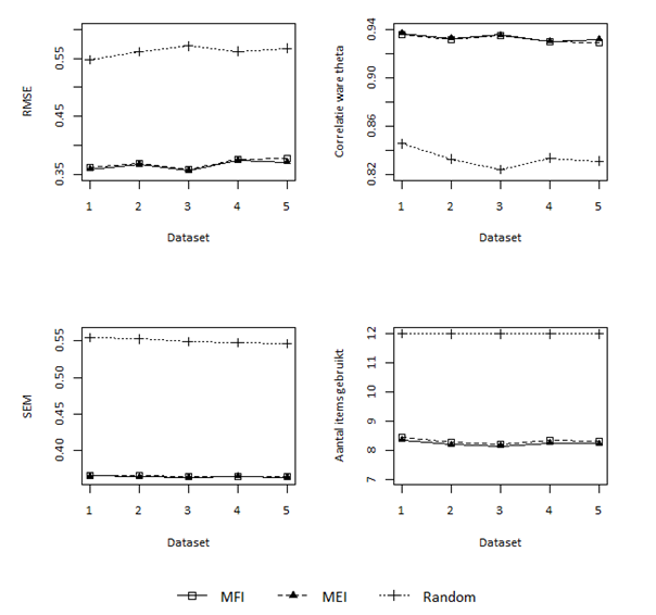
Figure 1.6. Comparison of different item selection methods for Verbal Analogies.

Figures 1.5 and 1.6 show that there are only minimal differences between the two item selection methods for both the Figure Sets and Verbal Analogies tests. We can see that both the MFI and MEI methods perform a lot better in comparison to the at random method. In general, the RMSE was slightly lower with the MEI method than the MFI method with Figure Sets, while the opposite was true in the case of Verbal Analogies. For both sub-tests, slightly fewer items were needed to obtain these more accurate measurements, but once more, these differences were nil. We decided to use the MEI method partly based on the findings of Van der Linden and Glas (2010) but also because this method is likely to yield more efficient measurements as soon as we collect enough data in the future to be able to use the 3PL model. Furthermore, the more efficient measurement of the MEI method will give a better estimate of θ if restrictions are imposed on the items that can be shown in the interests of exposure control. This will be explained in detail in section 1.7.
1.5.3. Starting rule/start θ
We chose to set the start θ at just under the average, at θ = -0.5. This gives people a better chance of answering the first item correctly, which will give them a better test experience. The consequences of this choice with respect to the more standard start value of θ = 0 were examined using simulation studies; the accuracy of the estimation of θ against true θ was not impaired by this decision.
1.5.4. Stopping rule
The most commonly used stopping rule in adaptive tests is stopping when SEM < x, whereby x is a criterion determined beforehand, therefore the degree of precision. We chose a value of 0.39, which theoretically corresponds to a reliability of .85 (1- 0.392 = 0.85; Thissen, 2000) for each of the three sub-tests. This is more than sufficient at sub-test level (> .80; Cotan, 2009) in tests to assist important decisions, such as personnel selection, the objective for which ACT General Intelligence was developed. We must note here that ACT General Intelligence consists of three sub-tests: the reliability of each sub-test separately is important to this, but what is even more important is the reliability of the total score calculated on the basis of all the sub-tests. If a sub-test has a reliability of .85, this is already high, but that of the total test will be higher still (see Chapter 5).
We have placed limits on this stopping rule by setting a minimum and maximum number of items, 7 and 12 respectively. The stop criterion can be reached quickly at around average θ values (around 0) – after all, there are many informative items in this area – but a person may give a few incorrect answers at the start that do not reflect their real θ. To rectify these ‘errors’ they will need more items. In order not to ‘punish’ people too severely for this type of error we initially set the minimum number of items at 7. To limit the time it takes to sit the test, we set the maximum number of items at 12 in the first version of ACT General Intelligence. Most people, however, will need fewer items to obtain a reliable estimate of θ (also see Chapter 5).
1.6. Specifications of ACT General Intelligence V1
- Each sub-test begins just under the average level (θ = -0.5)
- Items are selected on the basis of the Maximum Expected Information method
- θ is estimated on the basis of the expected a posteriori method (EAP).
- The minimum number of items is 7, the maximum number is 12.
- The test stops when SEM < .39 (unless fewer than the minimum number or the maximum number of items has been shown), which approximately corresponds to a reliability of .85 per subtest
1.7. Study of exposure control methods and ACT General Intelligence V2
1.7.1. Background underutilisation and overutilisation
The first version of ACT General Intelligence was made available in February 2015 and used by a number of Ixly’s clients for several months. In this version, approximately 40 items from the item bank were used for each sub-test. This is a direct consequence of the item selection method that was used. The most informative item is always chosen to give the quickest and most accurate measurement possible of θ: in practice these were the items with the highest discrimination parameters (a, see Figure 1.4). Consequently, a small number of items were overutilised, while a large number of items were underutilised.
This overutilisation and underutilisation of items is undesirable for a number of reasons, the most important of which is item familiarity. Items and their answers could become known through distribution on internet, which would obviously jeopardise the test’s reliability and validity. Another reason is the investment made in the item bank: it would be a waste to only use a small percentage of it. Thirdly, one of the main benefits of IRT models is that the difficulty and discriminatory power of items is known; this makes it possible to measure a person’s intelligence equally accurately using different items. It would be a waste not to make optimal use of this characteristic of IRT.
1.7.2. Methods to prevent underutilisation and overutilisation.
For all these reasons a number of methods have been developed in the literature to prevent the underutilisation or overutilisation of items, each with their own pros and cons (Veldkamp, 2010). A simple method, for example, is not to take the most informative item, but, say, the 5 most informative items and to choose 1 at random. Another commonly-used method is the Sympson-Hetter method (1985), but finding the correct control parameters for it is extremely time-consuming (Veldkamp, 2010). What’s more, these parameters must be recalculated each time a change is made to the item banks. Therefore, we did not use this method.
Another method is the Progressive-Restricted method (Revuelta and Ponsoda, 1998). This was initially designed to prevent the underutilisation of items and seems to be very successful in doing so (Veldkamp, 2010). The idea is simple: each time an item is chosen, the information that it provides is weighted using the following formula and the item with the highest value is shown:
(1.5)
whereby Ri is a random number between 0 and the information value of the most informative item for θ at that point in time, s is the number of items shown in the test up until that point and n is the maximum number of items in the test. The formula clearly reveals that at the start of the test, the random component is large and the information component is small, but that this situation is reversed as the test progresses.
The formula also shows that this method has a number of disadvantages: at the start of the test, candidates will receive an item from the item bank completely at random, which means that they may receive a very easy or a very difficult item. The latter will not be beneficial to the test experience. Furthermore, there is no check on overutilisation: it is questionable whether the goals regarding the maximum number of times that an item may be shown (for example ‘in 30% of the total number of tests’) will be achieved (Veldkamp, 2010).
1.7.3. Research into different methods
We have therefore used simulation studies to test variants of this Progressive-Restricted (hereinafter PR) method intended to remedy these disadvantages and examine the degree of exposure. In the first variant, the above formula is still weighted with the exposure rate (ER) of an item up to that point in time (i.e. the number of times the item was shown divided by the number of times the test was taken). Specifically, the above formula was weighted with 1-ER: if an item is shown in all cases (ER = 1), the result of the formula will therefore be 0 and the item will automatically not be shown. This adjustment restricts overutilisation. This method will be referred to hereinafter as 1-er PR.
The second type is the Fuzzy method developed by Ixly. This method combines a number of characteristics of different methods. Therefore, information for the first item is only weighted with 1 exposure rate: with the envisaged result that the first item is not shown randomly but is approximately around -0.5 (as in Version 1). Furthermore, the random component is reduced by adding a constant to the second part of the above formula (after the +). Finally, in order to prevent overutilisation, one item is chosen at random each time from the three items with the highest outcomes from the formula.
Clearly, a great many interests are at play simultaneously concerning the restrictions on displaying items: items may not be displayed too often, but still must be measured accurately; as many items as possible from the item bank must be used, but candidates must not be given items that are too difficult or too easy in the interests of the test experience; the test must be kept as short as possible, etc. All these points have been taken into account insofar as possible when determining the best method. We used the 40% target as the maximum exposure rate; therefore an item may not be shown in more than 4 out of the 10 tests used. As all three methods lead to less accurate measurements (the most informative item is no longer always chosen), we increased the maximum number of items to 15. This gives the test more ‘time’/opportunity to collect information on a person’s θ. The results concerning the accuracy of the measurement are shown in Table 1.4.
|
Table 1.4. Results of simulation studies into the utilisation of items: accuracy |
||||||||||||
|
RMSE |
Average SEM |
Correlation true θ |
Number of items |
|||||||||
|
Fuzzy |
PR |
1-er PR |
Fuzzy |
PR |
1-er PR |
Fuzzy |
PR |
1-er PR |
Fuzzy |
PR |
1-er PR |
|
|
Digit Sets |
.36 |
.36 |
.37 |
.36 |
.36 |
.37 |
.94 |
.94 |
.93 |
8.79 |
8.59 |
10.06 |
|
Figure Sets |
.38 |
.38 |
.39 |
.38 |
.38 |
.38 |
.93 |
.93 |
.92 |
10.03 |
9.60 |
12.12 |
|
Verbal Analogies |
.32 |
.33 |
.35 |
.32 |
.33 |
.35 |
.95 |
.95 |
.94 |
7.74 |
7.81 |
8.41 |
|
g score |
.23 |
.23 |
.25 |
.20 |
.20 |
.21 |
.98 |
.98 |
.98 |
26.56 |
26.00 |
30.59 |
|
Note: Values in the table are average values over the five simulated data sets. |
||||||||||||
The three methods differ little from each other with regard to the accuracy with which θ is measured. It is striking that relatively more items are required for the 1-er PR method than for the other two methods (over ACT General Intelligence in its entirety, therefore over the three sub-tests consisting of approximately 5 items) and that this does not lead to more accurate measurements. As one of the objectives was to keep the test as short as possible, this method was rejected.
Table 1.5 shows the results for the use of the item banks with the three methods. It is striking that both the PR and the 1-er PR methods leave almost no item unused. Using the Fuzzy method, this is 24% for the Digit Sets, 23% for the Figure Sets and 28% of the respective item banks.
|
Table 1.5. Results of simulation studies into the utilisation of items: use of the item bank |
||||||||
|
# Unused items |
Max ER |
Min/Max b 1st item |
||||||
|
Fuzzy |
PR |
1-er PR |
Fuzzy |
PR |
1-er PR |
Fuzzy |
PR + 1-er PR |
|
|
Digit Sets |
50.2 |
0.4 |
0 |
0.31 |
.45 |
.27 |
-.78/.08 |
-1.79/3.82 |
|
Figure Sets |
42.8 |
0.2 |
0 |
.40 |
.62 |
.39 |
-.77/.22 |
-3.64/3.87 |
|
Verbal Analogies |
60.4 |
1.2 |
0 |
.28 |
.31 |
.20 |
-.65/.20 |
-1.67/4.18 |
|
Note: The values shown in the table are average values over the five simulated data sets. |
||||||||
If we look at the maximum exposure rates we see that they are lowest with the 1-er PR method, but that the values differ little from the Fuzzy method. When using the PR method, the maximum exposure rate for two of the sub-tests > .40, which is too high. The distribution of the exposure rates for the Digit Sets is shown in Figure 1.7. The items are ranked by exposure rate from high to low. The figure shows that the exposure rates of the PR method are the most out of balance: there are items with quite high values and also a large number with lower values. The 1-er PR method shows the most homogenous exposure rates. The Fuzzy method is approximately somewhere in-between.
Figure 1.7. Item utilisation for Digit Sets – Simulation 1.

In the last columns of Table 1.5. we see that, because the first item is chosen at random, it can be any item from the item bank, including very easy or very difficult items. When the Fuzzy method is used, the difficulty of the items is around -0.50, as intended.
Conclusion
After taking all this into consideration, we chose the Fuzzy method to prevent both the underutilisation and overutilisation of items. The only disadvantage of this method is that part of the items from the bank remain unused, but this is more of a problem for Ixly (unnecessary investment) than for the candidates. The Fuzzy method is one of the best choices with regard to the exposure rates, and when other criteria are taken into consideration it is the best choice. Furthermore, the Fuzzy method does not pose any problems with regard to item familiarity. This method was therefore used in ACT General Intelligence V2.
Finally, we would like to comment on the content of the items using the selected control method. In adaptive tests, each candidate is shown different items. Therefore, it is possible that certain subjects are not adequately covered during the test. There are control methods that take this into account (see, for example Kingsbury and Zara, 1991) and ensure that all subjects are covered sufficiently. However, these possible limitations of adaptive tests play a larger role in tests where it is possible to clearly distinguish specific subjects or content domains. Take the example of an examination on Dutch history after 1945 which must contain questions on each decade (as opposed to only setting questions about the decade 2000-2010 and asking no questions about the other decades). Another example is a transition test for maths at a primary school where pupils must show that they have sufficient knowledge of fractions, multiplication and square roots (therefore they must not only receive questions about fractions).
This is less relevant in ACT General Intelligence because there are no specific content domains that must be questioned in equal measure. The sub-tests contain different logical rules that must be found, but there are also a lot of different rules that cannot be classified into specific content domains. We have therefore chosen not to use a control method with content control.
1.8 Recalibration and Version 3
Changes in Version 3
The second version of ACT General Intelligence was in use from July 2015 to July 2016. In July 2016, new analyses were conducted on items with new data (N = 2532, see Chapter 6 for more information on this sample) obtained in the previous periods during which the test was actually in use. These data were derived from clients of Ixly, who had used the test as part of their selection procedure. Once more, we calculated item fit statistics and listened to feedback from users on item content. Based on information obtained from these two sources, a number of items were removed from item banks for the Digit Sets and Figure Sets tests. Eventually, we were left with 122 items (including 6 ‘research items’) in the item bank for Digit Sets and 126 items (including 12 ‘research items’) for Figure Sets. The item bank for Verbal Analogies remained unaltered. All research results following on from this were obtained on the basis of item parameters – and the θs based on it – as established in the recalibration in July 2016.
The item parameters corresponded strongly to the parameters estimated on the basis of the calibration sample. The correlations between the a values on the basis of the old and new calibration were .92, .87, and .94 respectively for Digit Sets, Figure Sets and Verbal Analogies. The correlations for the b values were .98, .88 and .94 respectively. The average a values did not differ much from each other (old vs. new; 1.47 vs. 1.37 for Digit Sets, 1.01 vs. 1.02 for Figure Sets and 1.67 vs. 1.65 for Verbal Analogies). The same applied to the b values (.12 vs. -.05 for Digit Sets, .83 vs. .59 for Figure Sets and .67 vs. .43 for Verbal Analogies). In the new calibration, the difficulties were always estimated slightly lower (easier) than in the original calibration.
The influence of this was studied by correlating the θs based on the first calibration of the calibration sample with the θs based on the second calibration. These correlations were extremely high: .98, .96 en .94 for Digit Sets, Figure Sets and Verbal Analogies. The correlations between the SEM values were .98, .99, and .98 respectively.
Because the item banks for Digit Sets and Figure Sets were smaller and more informative for slightly lower levels (see Chapter 2) it was decided to raise the minimum number of items to 10 and the maximum number of items to 17. This makes it possible to produce an accurate measurement for the entire θ scale. A simulation study was conducted to research this. Analogous to the previous simulation studies, we simulated a sample of 1000 people / true θs from a normal distribution N (0.1) and generated response patterns. We did not simulate multiple samples as previous simulation studies had shown that the results for different simulated samples hardly differed from each other. We then simulated the adaptive test with the new setting with 1000 simulated candidates. The results are shown in Table 1.6.
|
Table 1.6. Results of simulation studies of characteristics of ACT General Intelligence after recalibration. |
||||||||
|
RMSE |
Average SEM |
r true θ |
Number items |
Min/Max b 1st item |
# Unused items |
Max. ER |
||
|
Digit Sets |
.35 |
.36 |
.94 |
11.48 |
-.81/-.12 |
0 |
.53 |
|
|
Figure Sets |
.37 |
.38 |
.93 |
12.99 |
-.80/.36 |
0 |
.46 |
|
|
Verbal Analogies |
.29 |
.28 |
.96 |
10.29 |
-.52/-.04 |
52 |
.24 |
|
|
g score |
.21 |
.19 |
.98 |
34.76 |
- |
- |
- |
|
Table 1.6. shows that the adjustments did not lead to a reduction in the qualities of ACT General Intelligence – in fact, if we take the RMSE, average SEM and correlation with the 'true’ θ, we can say that the test now produces slightly more accurate measurements than before (compare with Table 1.5., 'Fuzzy' columns). It is true that more items are needed to obtain this measurement, but with an average of approximately 35 items the test is still extremely short. Finally, we can observe that it can be expected that all items in the smaller item banks for Digit Sets and Figure Sets will be used.
2PL or 1PL model
When conducting the review in July 2016 it was examined whether the 2PL model was a better description of the data than the 1PL model. This is apparently the case according to the χ2 tests based on the -2loglikelihood values (see section 1.5.1.4.) and the lower BIC values of the 2PL in comparison to the 1PL model (lower values indicate a better model fit). However, we also looked at the relative efficiency (De Ayala, 2013) of the models. Relative efficiency tells us something about the information delivered by one model in comparison to another model. Specifically, we have calculated this as follows: for all θ values ranging from -3 up to and including 3 (in increments of 0.1) we have the total information as delivered by the item bank for Digit Sets, Figure Sets and Verbal Analogies respectively. We then calculated the Information (2PL)/Information (1PL) ratio: a ratio >1 means that the 2PL model provides more information over the entire θ scale than the 1PL model; a ratio <1 means that the 1PL model provides more information than the 2PL model. For Digit Sets the 2PL model provided approximately 10% more information than the 1PL model, while for Figure Sets and Verbal Analogies, the 1PL model gave more information than the 2PL model, 5% and 4% respectively.
Therefore, there might be some doubt as to whether opting for the 2PL model has an adverse effect on estimates of θ and the accuracy of ACT General Intelligence. A simulation study was conducted to investigate this. First, 1000 true θs were generated and answers were then generated on the basis of these θs according to the 1PL model (thus on the basis of the item parameters estimated with the 1PL model) and according to the 2PL model. Four conditions were then simulated:
- A condition with answer patterns according to the 1PL model, whereby the adaptive test used the item parameters of the 1PL model
- Answer patterns according to the 1PL model, whereby the adaptive test used the item parameters of the 2PL model
- Answer patterns according to the 2PL model, whereby the adaptive test used the item parameters of the 2PL model
- Answer patterns according to the 2PL model, whereby the adaptive test used the item parameters of the 1PL model
Thus we examined the impact of a deviation from ‘reality’ (for example if response patterns are based on the 1PL model in practice, but estimated in the adaptive test using the 2PL model) on the outcomes of ACT General Intelligence. This made it also possible to compare whether the 1PL model simply did not lead to better outcomes than the 2 PL model (comparing condition 1 and 3).
The results of this study are shown in Table 1.7.
|
Table 1.7. Results of simulation study with respect to the suitability of 1PL versus 2PL. |
||||||||||||||||||||||||
|
RMSE |
Average SEM |
Correlation true θ |
ER |
Number of items |
||||||||||||||||||||
|
1 |
2 |
3 |
4 |
1 |
2 |
3 |
4 |
1 |
2 |
3 |
4 |
1 |
2 |
3 |
4 |
1 |
2 |
3 |
4 |
|||||
|
Digit Sets |
.39 |
.48 |
.35 |
.49 |
.39 |
.36 |
.36 |
.39 |
.93 |
.88 |
.94 |
.88 |
.83 |
.83 |
.85 |
.81 |
16 |
11 |
11 |
16 |
||||
|
Figure Sets |
.43 |
.51 |
.37 |
.52 |
.42 |
.38 |
.38 |
.42 |
.91 |
.87 |
.93 |
.87 |
.79 |
.80 |
.84 |
.74 |
17 |
13 |
13 |
17 |
||||
|
Verbal Analogies |
.38 |
.40 |
.29 |
.45 |
.38 |
.27 |
.28 |
.38 |
.93 |
.92 |
.96 |
.91 |
.84 |
.90 |
.91 |
.79 |
11 |
10 |
10 |
10 |
||||
|
g score |
.27 |
.34 |
.21 |
.38 |
.23 |
.19 |
.19 |
.23 |
.97 |
.96 |
.98 |
.95 |
.90 |
.82 |
.95 |
.77 |
44 |
34 |
34 |
43 |
||||
|
Note: 1 = 1PL with 1PL, 2 = 1PL with 2PL, 3 = 2PL with 2PL, 4 = 2PL with 1PL. |
||||||||||||||||||||||||
|
ER = empirical reliability |
||||||||||||||||||||||||
The results show that the 2PL model delivers the best outcomes: it best approaches the true θ as demonstrated by the lowest RMSE values and the highest correlations with the true θ. Furthermore, the 2PL model needs relatively few items to achieve this. A comparison of conditions 1 and 4 shows that when the model used for the ACT General Intelligence conforms to reality (i.e. 1PL-1PL or 2PL-2PL), the 2PL model gives a better estimate. At the same time, a comparison of conditions 2 and 4 shows that a deviation from reality (i.e. 2PL-1PL or 1PL-2PL) affects the estimate of θ more adversely if the answers follow the 2PL model in practice after outcomes have been estimated using the 1PL model than the other way around. In the case of the former, for example, empirical reliability (condition 4) is lower than in case of the latter (condition 2), while the average SEM is higher. The RMSE values and correlation with the true θ differ little from each other; however, the number of items in the fourth condition is considerably higher than in the second condition.
Conclusion
This simulation study has shown that in ACT General Intelligence, the 2 PL model is a better description of reality than the 1 PL model. This study therefore justifies the choice of the 2PL model to estimate the item parameters of the three sub-tests, Digit Sets, Figure Sets and Verbal Analogies.
1.9 Specifications of ACT General Intelligence V3
- Each sub-test begins just under the average level (θ = -0.5)
- Items are selected on the basis of the Maximum Expected Information method
- θ is estimated on the basis of the expected a posteriori method (EAP)
- The minimum number of items per sub-test is 10, the maximum is 17
- The test stops when SEM < .39 (unless fewer than 10 items or 17 items have already been shown), which approximately corresponds to a reliability of .85 per subtest
As item calibration was performed on the total sample (calibration sample and candidate sample from the Ixly database), all results for this total sample will be discussed, in addition to the candidate sample. We opted for this approach because in the first place it is important to gain insight into the psychometric qualities of the items and scores in the group on which the item parameters are based. However, because there are also people in this group (namely those from the calibration sample) who have not taken the test adaptively, but under different circumstances than 'real' candidates, it is also important to provide insight into the characteristics of the test with regard to the latter group. Direct users of the test will attach greater importance to the results for candidates who have taken the test in selection situations.
1.10 Colour information and the ACT General Intelligence V4
Changes in version 4: Colour perception and colour blindness
Background
Not everyone perceives colour in the same way. People who have difficulty with colour perception are not always able to recognise or distinguish between certain colour combinations (Tanaka, Suetake & Uchino, 2010). To check whether colour blindness could affect users of ACT General Intelligence, a study was conducted into the various types of colour blindness. This revealed that the two most common types of colour blindness are protanopia and deuteranopia. In people suffering from protanopia, the ‘red’ cone type in their eyes is either defective (protanomaly) or totally absent (protanopia). In people with deuteranopia, the ‘green’ cone type is either defective (deuteranomaly) or absent (deuteranopia) (Tanaka et al., 2010). In both cases, subjects find it difficult to distinguish between colours in the green-yellow-red section of the colour spectrum (Tanaka et al., 2010). Protanopia occurs in 2.13% of the Dutch population, while deuteranopia occurs in 5.28%. The other types of colour blindness occur in less than 0.01% of the Dutch population (Accessibility.nl, 2020).
Implementation
To ensure that colour blindness (whether protanopia or deuteranopia) does not present an obstacle to anyone using ACT General Intelligence, we examined each component to ascertain whether colour perception might influence a candidate’s performance for the revised version of februari 2020. Colour perception does not have any influence on the performance of candidates in either the Digit Sets or Verbal Analogies sub-tests. The Figure Sets sub-test, however, frequently uses multiple colours to indicate a distinction. Each item in this sub-test was assessed to ascertain whether an inability to distinguish between colours could present a problem for colour-blind candidates with protanopia or deuteranopia. This assessment was done using the RGBlind extension, an open source, real-time colour-blindness simulation tool, developed to overcome problems caused by protanopia or deuteranopia. Using the RGBlind extension enabled us to assess whether the items containing several colours had enough contrast to be used by candidates with protanopia or deuteranopia (Accessibility.nl, 2020). We identified 7 items in the third version of the ACT General Intelligence that could potentially pose a problem for people with these types of colour blindness. The question and answer options in these items (34 pictures in total) have therefore been adapted in the revised version of februari 2020, to ensure that candidates should be able to distinguish between the colours used. This was accomplished by selecting colours at the extreme ends of the colour spectrum, such as blue-red-yellow or green-pink. The changes were then verified using the RGBlind extension. According to this verification, the colours ultimately selected were sufficiently distinctive. These changes ensure that the fact that a person with protanopia or deuteranopia perceives colours differently will not influence their performance in ACT General Intelligence.
2. Test Material
2.1 Introduction
This chapter will discuss the test material used in ACT General Intelligence. First of all, we will examine the characteristics of the items and item banks used for the sub-tests. We will then look at how the test is taken, ways in which the software may be used incorrectly and the scoring system.
2.2 Characteristics of the items and sub-tests
2.2.1. Digit Sets
Below is an example of a Digit Sets item.
Figure 2.1. Example of an item in a Digit Sets test.


Candidates sitting a Digit Sets test are required to recognise a logical pattern in a series of numbers. According to this logic, they must work out which number should replace the question mark. In this case, the logic is as follows: the first number is multiplied by six, the second by five, the third by four, the fourth by three; this must lead to the conclusion that the fifth number should be multiplied by two, and therefore the answer is 1440. This means that the third option is correct.
This is just one example of the many logical connections that test subjects may be asked to uncover: in some items, each number must be multiplied by a constant, in other items a smaller or larger number must be subtracted or added, etc. Some items actually have two series hidden within them, so that the candidate must realise that the series keeps skipping a checkbox.
Figure 2.2 shows the information value and accompanying SEM of the entire Digit Sets item bank containing 122 items. It shows us that although the items are most informative when θ is set at approximately -1.5, there are still enough discriminating items between -1 and 1 (see next section). The a parameters range from .22 up to and including 3.94, with an average of 1.37. The higher the discrimination value, the better: values of .80 or .90 or higher are regarded as good discrimination values (Swartz & Choi, 2009). There are 79 items with an a > .90, which is approximately 65% of the items. The b parameters have a minimum of -2.17, and a maximum of 4.44, with an average of -.05.
Figure 2.2. Digit Sets Itembank

In Figure 2.3. the difficulties (b) of items are plotted against their discrimination values (a). The items are mainly clustered in the middle and slightly less difficult items generally have higher discrimination values (this is also to be expected on the basis of Figure 2.2). In selection situations, it is particularly important to have a sufficiently accurate measurement in the area from -1 up to and including 1. There are 53 items in this area, 35 (66%) of which have an a value greater than or equal to .90. From this, we can conclude that the Digit Sets item bank contains good items that are sufficiently discriminating.
Figure 2.3. Discrimination (a) and difficulty (b) parameters for the Digit Sets.

2.2.2. Figure Sets
Below is an example of an item from the Figure Sets test.
Figure 2.4. Example of an item in a Figure Sets test.

In this item, candidates must examine the eight squares that have been filled in to find which of the four options fits in the empty square on the bottom right. In this case, the candidate should see that each column and each row has one round face, one square face and one face without an outline. In the right-hand column and bottom row there is no face with a round outline. All four answers meet this criterion. Each column and each row has a happy mouth, a straight mouth and a crooked mouth. Therefore answer B is not correct. Finally, each column and each row has one face with open eyes, one face with dashes for eyes and one face with arched eyes. From this, we can conclude that answer A is correct.
Several of the items in the Figure Sets follow this format, but there are many more item types. In some cases, the matrix is a complete continuous picture that must be completed by the candidate. In other cases, objects in rows or columns must be added up or subtracted and the candidate must uncover this pattern.
Figure 2.5 shows the information value and accompanying SEM of the entire Figure Sets item bank, consisting of 126 items. From this, it is clear that the items are most informative when θ is approximately -1.5 to -1, whereby it can be observed that items do not differ greatly from each other between -1.5 and 1 with regard to the information they supply (the SEM line is reasonably flat in this range). The a parameters range from .25 up to and including 3.46, with an average of 1.02. There are 62 items with an a >.90, which is approximately half of the items. The b parameters have a minimum of -2.18 and a maximum of 4.43, with an average of .53.
Figure 2.5. Figure Sets Itembank.
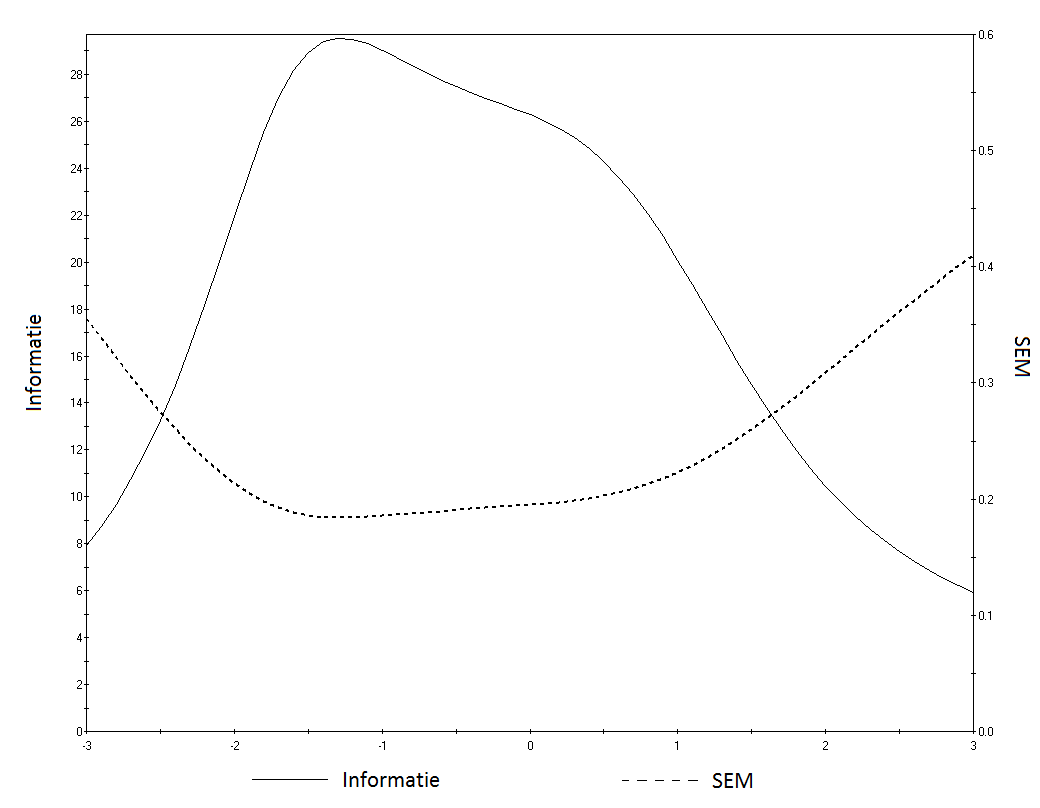
In Figure 2.6., difficulty (b) is once more plotted against the discrimination values (a) of the items. The item bank contains more difficult items than easy items. The items that are of more average or lesser difficulty are also more discriminating.
There are 59 items in the area between the θ values -1 and 1, 41 (69%) of which have an a value greater than or equal to .90. From this, we can conclude that the Figure Sets item bank contains good items that are sufficiently discriminating.
Figure 2.6. Discrimination (a) and difficulty (b) parameters for the Figure Sets.

2.2.3. Verbal Analogies
Below is an example of an item from the Verbal Analogies test.
Figure 2.7. Example of an item from the Verbal Analogies test.

The items in Verbal Analogies feature words that are related to each other, presented in a square. Candidates must recognise the connection between the two words already filled in (the analogy) and complete it by choosing two words from the available options or by finding two words in the options given that bear the same relationship to each other as the two words already filled in. The above example is a case of the latter. You use your feet to walk and your eyes to read. Therefore ‘read’ and ‘eyes’ are the correct answers.
Once more, this is only one example as there are many connections that can be discovered between words, such as contradictions, synonyms, part of the same, user of, maker of, product of, etc.
Figure 2.8 shows the information value and accompanying SEM of the entire Verbal Analogies item bank consisting of 214 items. The peak of the information curve is around .50, which means that the items are most informative when θ is 0.50. The a parameters range from .27 up to and including 4.42, with an average of 1.65. There are 168 items in total with an a > .90, so approximately 79% of the items. The b parameters have a minimum of -2.46 and a maximum of 4.27, with an average of .43.
Figure 2.8. Verbal Analogies Itembank.
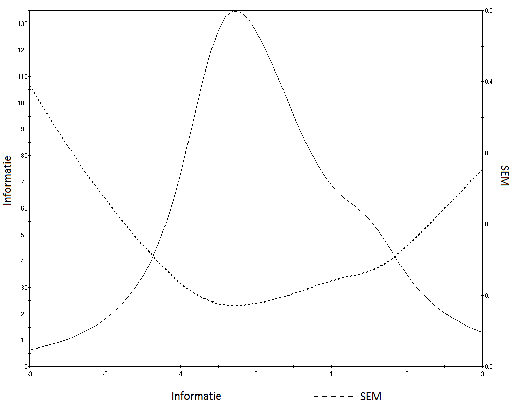
Figure 2.9 shows that more difficult items generally have lower discrimination values, as is the case in the other two sub-tests. The most discriminating items are around the average, ranging between -0.5 and 0.5.
There are 139 items in the area between the θ values -1 and 1, 123 (88%) of which have an a value greater than or equal to .90. From this, we can conclude that the Verbal Analogies item bank contains items that are sufficiently discriminating within the range that is relevant for test purposes.
It is interesting that a number of extremely discriminating items can be found when θ is 1.5. This is expressed in Figure 2.8 by the small ‘bump’ around this θ in the information graph.
Figure 2.9. Discrimination (a) and difficulty (b) parameters for Verbal Analogies.

2.3. Characteristics of ACT General Intelligence in its entirety
When we look at the three item banks in Figures 2.2., 2.5. and 2.8., we see that with regard to difficulty, the three sub-tests are well distributed around the θ values where the most discriminating items are found. This is around a θ-value of -1.5 for Digit Sets; a wide range from approximately -1.5 to 1 for Figure Sets and between -0.5 and 0.5 in the case of Verbal Analogies. This means that, taken together the three tests cover the relevant θ values thoroughly. Having said this, we must pay attention to the fact that the emphasis is on the lower levels in Digit Sets and Figure Sets. Therefore, we will develop and research more and more highly discriminating items at higher levels for these sub-tests in the future.
If we compare the discrimination values, the information values and the SEM values of the item banks belonging to the three sub-tests, we see that the items from Verbal Analogies are 'the best': the information values are highest for this item bank (therefore the SEM values are the lowest over the entire θ scale). The items from the Figure Sets provide the least information. It is important to note hereby that these sub-tests ultimately produce a g score: although a measurement given by a sub-test will be more or less reliable individually, the estimate of the g score will be extremely reliable because it is based on three sub-tests (also see Chapter 5, Reliability).
In order to gain more insight into this, the information and SEM values of ACT General Intelligence’s total item bank (therefore all items in the Digit Sets, Figure Sets and Verbal Analogies together) are shown in Figure 2.10. This figure shows that, on the whole, most information is found at average θ values (the minimum is approximately -0.5), and that the least information is found at extremely high or, conversely, low θ values. In general, however, we may conclude that there is enough information available to enable us to measure the entire θ scale accurately (see Chapter 5).
Figure 2.10. Total Itembank of ACT General Intelligence

With regard to fluid and crystallized intelligence, the g score mainly measures fluid intelligence: as explained earlier, the characteristics of the items limit the influence of crystallized intelligence insofar as possible. In the literature, measurements of g are also considered as measurements of fluid intelligence and the g score determined on the basis of ACT General Intelligence is no exception.
2.4 Instructions for conducting the test
2.4.1. Conducting the test
All questionnaires made available by Ixly are administered in the Test Toolkit (see Figure 2.11). This online application gives professionals and consultants in the field of Human Resource Management a set of qualitative tools. In principle this portal can be accessed from any computer or laptop and in any browser. Consultants can log in with a user name and password. They can then add a candidate to the system and allocate various tests to them, including ACT General Intelligence. After allocating the test, the consultant can invite the candidate to take it. The candidate will receive the invitation in an email containing a unique link to the test environment.
Please see appendix 2.1 for the consultant’s guide. There is more information on operating the test portal at http://www.ixly.nl/kennisbank/test-toolkit-tutorial/ and http://www.ixly.nl/kennisbank/test-toolkit-faq/.
Figure 2.11. Overview screen for candidates.

Instructions
When a candidate clicks on the unique link in their email, they will be sent to a test environment containing all the tests allocated to them. They will start with an opening questionnaire which asks them to provide information about background variables such as age, gender and education. This information will only be used for research purposes. Candidates are given clear instructions before starting ACT General Intelligence.
Figure 2.12. Instructions - Screen 1.

Figure 2.13. Instructions - Screen 2.

Because research has shown that explaining how an adaptive test works is important for the candidate’s test experience (also see Chapter 1, section 1.4.1.), we have chosen to do so in the instructions (see Figure 2.12., instruction screen 1). To ensure that everyone can understand the text (in line with our goal of culture-free testing) the explanation is brief and written in plain language devoid of any technical or statistical terms. Other points mentioned include (see Figure 2.12 and 2.13):
- That each sub-test is preceded by a sample exercise and three practice exercises
- The time for each item (45 seconds)
- The approximate total test time (40 minutes, but usually shorter)
- When they can pause it
- Missing answers will be deemed incorrect
- Candidates can use a paper notebook when taking the test
Sample exercise and practice exercises
Each sub-test is preceded by a sample exercise and three practice exercises. The sample exercise for the Digit Sets is shown in Figure 2.15.
Figure 2.15. Sample exercise for the Digit Sets.
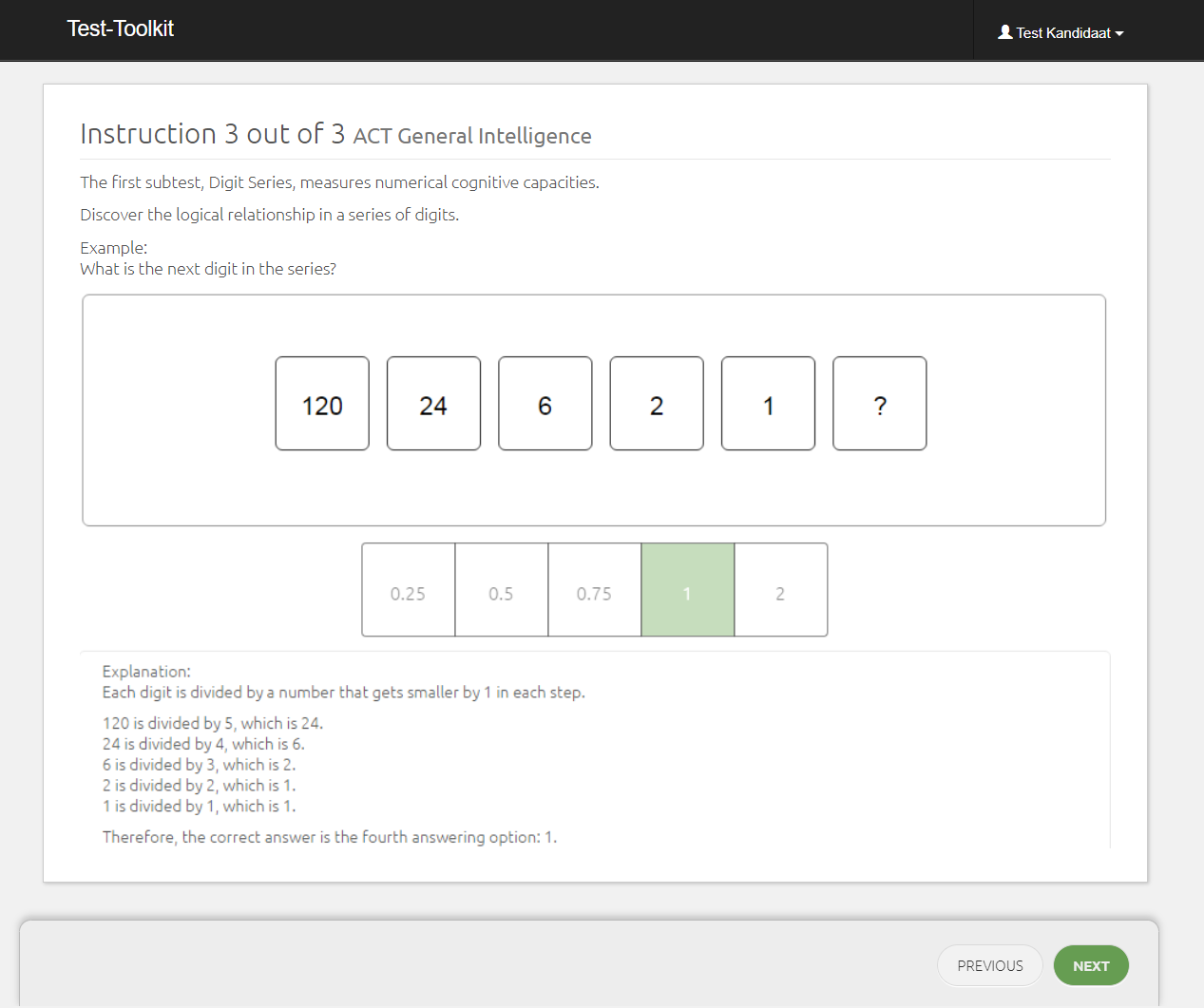
An explanation of the correct answer is given along with the sample exercise (Figure 2.14). Candidates doing a practice exercise are only told if their answer is correct or incorrect. Although it is known that giving feedback helps candidates to understand what is expected of them, there are several reasons to assume that they have been given sufficient information to be able to understand the test:
- They are given a sample exercise with an explanation of the answer.
- The sample exercises do not have a time limit, so that candidates can take as long as they want over them.
- The message ‘Unfortunately, this answer is incorrect’ or ‘This is the correct answer’ remains on the screen, giving candidates as much time as they want to understand why their answer was correct or incorrect.
- By finding this out and uncovering the logic behind it – which is also what they’re supposed to do in the sub-test, after completing the practice exercises – the candidate is training for the ‘real’ test.
The practice exercises are followed by an interim screen to inform the candidate that the sub-test will begin on the next page (Figure 2.16).
Figure 2.16. Screen for sub-test.

After every sub-test, an interim screen will appear to tell the candidate that they can take a short break and that the instructions for the next sub-test begin on the next page (Figure 2.17).
Figure 2.17. Interim screen.

At the end of the test, candidates are asked to click ‘Complete’ so that the results can be saved. They will then be referred to their overview screen where they may start on any other tests they may be taking. The consultant can then request the candidate’s report in their overview of candidates (see Chapter 3).
2.4.2. Preventing incorrect use of the software.
Test users do not have to take any further precautionary measures to prevent errors. For example, it is not necessary to close other programmes when taking the test. It is also not necessary to take any of the precautionary measures mentioned by Cotan (2009) (disabling unnecessary functions and hot keys, closing access to the hard disk and making it impossible to start other (unintended) software), as these will not have any effect on taking the test and the scoring. This also means that the influence of external factors on taking the test is limited and therefore the circumstances for taking the test will be practically the same for everyone. There are, however, a number of minimum system requirements which will be discussed in Chapter 3, Guide for test supervisors.
ACT General Intelligence was developed for selection purposes. For several years, there has been a trend for companies to allow candidates to take tests at home in the early stages of the selection process. These candidates therefore take the test in an unsupervised (unproctored) environment. This is in contrast to proctored tests, which are taken in an examination room in the presence of a test supervisor. As the ACT General Intelligence test is taken by computer/internet, users can decide whether they want candidates to take it in a supervised or an unsupervised setting.
Although this choice is up to the user, we would like to take a closer look at some of the aspects to be considered when making this decision. Apart from the practical, legal and ethical objections that have been expressed, there are also concerns about the validity of test scores obtained in an unproctored environment (Tippins et al., 2006; Pearlman, 2009). The main threat to test scores obtained under such conditions is the opportunity to ‘cheat’: for example candidates could get help from a friend, look up the answer on internet or even have another person take the entire test (Tippins et al., 2006). Interestingly, some studies have found no differences between scores obtained in supervised and unsupervised situations (Oswald, Carr, & Schmidt, 2001), other studies have found that scores were higher in unsupervised situations (Beaty, Fallon, & Shepherd, 2002; Do, Shepherd, & Drasgow, 2005) and yet other studies have found that scores were higher in supervised situations (Shepherd, Do, & Drasgow, 2003; Nye, Do, Drasgow, & Fine, 2008). Recent studies, however, seem to indicate that the validity of unproctored test scores is not in jeopardy, even in ‘high-stakes’ situations such as selection procedures, and that this also applies to cognitive tests (Arthur, Glaze, Villado, & Taylor, 2010; Beaty, Nye, Borneman, Kantrowitz, Drasgow, & Grauer, 2011; Kantrowitz & Dainis, 2014).
There do seem to be optimal conditions that best guarantee the validity of unproctored tests (i.e. that minimise the risk of ‘cheating’). For instance, the risk is smaller if an unproctored test is not too long (Tippins et al., 2006). Research has also shown that differences are minimised if items have a time limit (Kantrowitz & Dainis, 2014; Tippins et al., 2006). It is also a good idea to include an approve test to confirm the scores obtained and therefore the identity of the candidate from the unproctored test (Tippins et al., 2006). Adaptive testing, whereby each candidate may, in principle, receive a different test, also means that it makes less sense for candidates to look up answers. Having a large item bank also reduces the risk of item familiarity. In this way, adaptive testing can make tests safer and more reliable (De Ayala, 2013; Kantrowitz & Dainis, 2014).
ACT General Intelligence fulfils the aforementioned conditions, therefore it is reasonable to expect that the validity of the scores obtained will not be jeopardised. ACT General Intelligence items have a time limit and are adaptive. Furthermore, the test is relatively short, taking approximately 30 to 40 minutes to complete. There is also an approve test to confirm the candidate's identity. Theoretically, it would be possible to take screenshots of the items and share them with others later on, but as different people will receive different items the effect of this would be negligible.
Of course, a candidate could close the test in-between in order to gain time but this would not yield any direct benefit as the time allocated for the item would keep ticking. If a candidate has left the questionnaire half-way (which we advise against in the instructions), they may, in principle, re-start it via the link in the invitation email. They will then see an overview screen with a ‘continue’ button behind the title of the questionnaire. The candidate will then not continue where they left off, but the clock keeps ticking until the next task appears. This means that it is not possible to spend longer on an assignment than the time allotted for it.
Obviously, the candidate cannot return to previous assignments (nothing happens if you press ‘Previous’ in the browser). Once an answer is given, it is stored in the data base and can no longer be changed. All of the aforementioned test characteristics, instructions and the design of the test system limit the influence of external factors on scores to a minimum.
2.4.3. Scoring system
The exact way in which the adaptive procedure works – in other words, how a candidate’s answers lead to an estimate of their intelligence – is described extensively in Chapter 1. It explains the choices and justifications for the start, item selection and stop procedures of ACT General Intelligence.
The process for converting raw scores (correct/incorrect) to θs and then into standard scores is fully automated. Therefore, no errors can occur due to an incorrect interpretation by the test supervisor. To prevent errors due to incorrect input by Ixly’s test developers, strict procedures are followed before a test or questionnaire is made available to clients. These procedures are described in the quality manual drawn up within the framework of ISO 9001 certification. In short, this procedure means that the test is extensively tested before publication and during this process, checks are conducted to ensure that at each step in ACT General Intelligence (1) the information values of the items – on which item selection is based – are correct; (2) the θ is being calculated correctly and (3) the SEM is being calculated correctly. This is checked by comparing the above points from the Ixly test system with results from R, in which ACT General Intelligence can be simulated. It should be noted here that testing an adaptive test with a randomisation algorithm for item selection is more challenging than testing a ‘normal’ linear test. Unfortunately, the random element makes it impossible to set up a standard test protocol. A test file is available for checking this conversion from θs to the g score and the standardised scores.
The procedure is carried out by different developers. One developer takes the test in the Ixly online test system and a second developer checks the results in R and whether the θs are being correctly converted to the g score and the standardised scores. Once the procedure has been completed without any errors, the questionnaire is made available to clients.
2.4.4. Securing the test, test material and test results
Earlier, reference was made to the characteristics of ACT General Intelligence that guarantee the validity of the test results. Certain features of the test system also contribute to this objective.
A consultant prepares the questionnaire for the candidate. Candidates receive a unique link in an email with which they can log into the system. The consultant is responsible for entering the correct email address so that the link is sent to the candidate.
The management module where the data are stored, as well as the item parameters and item banks, can only be accessed by Ixly R&D staff using a unique combination of username and password that is changed regularly.
After the candidate has completed the questionnaire, the consultant will be notified that the results are available. The report containing the results is available in the consultant’s environment and can only be accessed using that consultant’s unique combination of username and password. We give consultants the opportunity to make the report immediately available to the candidate. However, this is not standard procedure and is up to the consultant. We also give consultants the opportunity to adjust texts in the report, but the scores, can never be altered.
Ixly has been ISO 27001 certified since 2014. This means that strictly confidential information is handled according to certain guidelines and ensures that the test results are guarded securely. All data are stored anonymously and ‘encrypted’ in a protected database with SSL certificates and this database is stored on a different server than the web application. External parties (such as software developers) work with anonymous data, which guarantees candidates’ privacy.
Ixly’s ISO 27001 certification also means that an external audit is held each year and a risk analysis and continuity plan are drawn up every quarter. Furthermore, data integrity and security incidents are monitored continuously. For more information on the contents of ISO 27001, go to http://searchsecurity.techtarget.co.uk/definition/ISO-27001.
3. Guide for test users
3.1. Introduction
This chapter will discuss the application, interpretation and use of ACT General Intelligence. We will look at the test’s applications and limitations, and the knowledge required to interpret the scores. We have also taken a few case studies to illustrate how test scores are interpreted.
3.2. Applications of ACT
ACT General Intelligence was primarily developed for selection purposes, but may in principle be used in any situation in which it is important to discover more about a person’s intellectual capacities. In line with the test’s principle objective, it is primarily intended for members of the Dutch working population. ACT General Intelligence gives a picture of a person’s general intellectual capacities (the g score) and more specifically of their numerical (Digit Sets), figurative (Figure Sets) and verbal (Verbal Analogies) capacities This gives users an idea of a candidate’s suitability for the job in question.
Although ACT General Intelligence was primarily developed for selection purposes, it can also be used for other assessment objectives, such as career-related issues that make it necessary or desirable to assess cognitive abilities. If, for example, a person is stuck in their career and would like to explore their options for career advancement or additional training together with a career coach, assessing their intelligence level will reveal or exclude certain options. ACT General Intelligence is a useful tool for gaining insight into a candidate’s cognitive abilities in such a situation. Section 3.6.3. features two case studies which explore this in greater detail.
3.3. Limitations
ACT General Intelligence has not yet been tested among school populations aged 15 and younger. Research must show whether ACT General Intelligence can also be applied to this age group. It would be a useful supplement to existing knowledge if more information on this was available. Although these groups do not fall under the target group (working population), ACT General Intelligence could still be applied to them.
3.4. Instructions for the test supervisor
The instructions provide all the information that a candidate needs to take the test. If the test supervisor wishes to provide information on taking the test beforehand, they can tell candidates the following:
- The test gives an idea of your intellectual capacities. Three sub-tests measure your numerical, abstract and verbal capacities and together they produce a general intelligence score for you.
- The test takes a maximum of 40 minutes in total, but usually takes less time to complete.
- Each sub-test is preceded by an explanation consisting of a sample exercise and three practice exercises.
- You will have 45 seconds to answer each question. Enter an answer before this time elapses. If not, the answer will be judged as being incorrect.
- We advise you to complete the test in one go. If, however, you have to interrupt it, you can do so after completing a sub-test. This is stated on the relevant screens.
- Only take the test if you have plenty of time to do so; leave at least 45 minutes free for it, and preferably an hour.
- Take the test in a quiet environment where you can concentrate.
- You may use a note pad during the test.
- Press F11 before starting the test to work in a full screen. Press F11 again to close the full screen.
Candidates must have some basic computer skills to be able to take the test. They must be able to:
- find an internet page via the browser;
- enter the username and password in the log-in page;
- use the mouse or keyboard to navigate through the portal (for example, to click on the start button, the answer options and next).
Font size, contrast and colours can be adjusted using standard browser settings to assist candidates with a visual disability. Candidates may also choose to only answer questions using a keyboard if it is difficult for them to use a mouse.
No further specific knowledge or training is required of candidates. Candidates do not have to practice before they take the test, but naturally this is possible. Ixly does not provide practice or sample exercises specifically for ACT General Intelligence. Ixly’s website has several sample tests that candidates may consult, but we leave this up to the candidates themselves or to consultants who may wish to inform candidates of this. The instructions that candidates read before taking the sub-tests contain a sample item and practice exercise as described above. The information given by the test supervisor and the sample and practice exercises ensure that candidates have enough information to be able to take the test.
3.5. Required knowledge for using the test
If ACT General Intelligence is being used by a professional to advise others or select them for a job, it is necessary to guarantee that this person:
- is competent, qualified, licensed or authorised to use psychological tests in the field in which they are employed for objectives such as assessment, coaching, training and Human Resource Management, the field in which they are employed. All this must comply with the legislation and regulations applicable in that country;
- will act and use the product in conformity with national or international professional standards and professional ethics.
- will act and use the product in conformity with national or international legislation and regulations, instructions and guidelines and all other applicable government or semi-government regulations;
- will only use the product for the organisation that employs them or their own company on their own behalf and on their own account. It is forbidden to sell, lease, copy, give, hand over or transfer the product in any way whatsoever or to any person or company whatsoever, unless the use of the products and services is an integral part of the service to clients or is designated for use within the organisation that directly employs them.
Ixly checks the reliability and knowledge of these professionals before granting access to its services and products. Ixly reserves the right to refuse a person access without stating reasons.
Although users do not have to be certified, we emphatically recommend that they follow training in test interpretation from Ixly before using ACT General Intelligence for consultancy matters within a professional context. Ixly gives training sessions approximately once every three months. These training sessions cover relevant theories on intelligence and personality, the construction and structure of Ixly’s most important tests, and interpretation of the results.
3.6. Interpreting scores
3.6.1. Calculating sub-test scores and the g score
The way in which the θs from the sub-tests are established is dealt with in Chapter 1: we use the EAP method to calculate θ. The scores for the three sub-tests can be derived from these scores.
Although these specific scores are interesting, in practice, people will mainly want to use the g score, partly because of its ability to predict work-related outcomes such as job performance (Schmidt & Hunter, 1998). The g score is calculated by taking a weighted average of the three θ scores based on the sub-tests: this weighting is based on the reliability of the sub-test scores. The idea behind this is that less reliable measurements (sub-test scores) are given less weight in the calculation of g and that this will give the most reliable measurement of g. The g score’s SEM (standard error) is calculated by adding up the information (= 1/SEM2) provided by the three sub-tests and calculating the SEM once more with this (= 1/√Info).
These calculations also assume that the three sub-tests belong to the same domain: i.e., that all three are a measurement of the same construct. If this is not the case, the information values should not simply be added up. This assumption is confirmed by the inter-correlations between the sub-tests and the fact that these could be explained by one factor (see Chapter 6).
3.6.2. Feedback of scores
The scores for ACT General Intelligence are fed back from four measures: the sten score, T score, percentile score and IQ scores (numerical, abstract, verbal and total). The main advantage of θ is that it is a normally distributed score. Therefore it is easy to convert it to other standard scores. Standard scores give an impression of a score in relation to the average of all scores within a certain reference group: an 'average' score is therefore a score that occurs often in the reference group, while a very high (or low) score means that this is rare in the reference group. We have used the following education levels: education level 2: lower secondary school; education level 4: post-secondary education; education level 6: bachelor or equivalent and education level 7: master or equivalent (known as VMBO, MBO, HBO and WO respectively in the Dutch education system) as reference groups for sten scores, T scores and percentile scores, and the working population as a reference group for the IQ score (see Chapter 4). For the sten scores and the IQ scores, the SEM is used to indicate the 80% confidence interval, graphically or in text ("We can say with 80% certainty that your total score is between X and Y").
The four raw scores of ACT General Intelligence – the θ-scores for the Digit Sets, Figure Sets and Verbal Analogies sub-tests and the g score, are first converted to a Z score and then to a sten score, T score and percentile score using the average and standard deviations of the four norm groups according to education level (see Chapter 4). The IQ score is calculated using the average and standard deviation of the working population reference group.
The consultant can request an extensive report, whereby they can opt for comparisons with one or more norm groups. Usually, the report only contains the IQ scores for the numerical, abstract and verbal elements and for the total. There is also a report available without these IQ scores, containing only the comparisons with the norm groups on the basis of education level. For a sample report, see appendix 3.1.
3.6.2.1. Sten score
This scale ranges from 1 to 10. Sten scores are a form of standard scores with an average of 5.5 and a standard deviation of 2. They give an impression of a score in relation to the average of all scores. Sten scores 4, 5, 6 and 7 are all within 1 standard deviation from the average. Sten scores 2, 3, 8 and 9 are all between within 1 and 2 standard deviations from the average. Sten scores 1 and 10 are more than 2 standard deviations from the average. The average score in the norm group is exactly on the border between the fifth and sixth sten. It must be noted here that sten scores must not be confused with school scores. A sten score of 5, for example, is not a fail, but means an ‘average’ score that is common in the reference group. The percentages for the separate sten scores are as follows:
|
Table 3.1. Sten scores with accompanying percentages |
||
|
Sten |
Percentage |
Cumulative percentage |
|
1 |
2.3% |
2.3% |
|
2 |
4.4% |
6.7% |
|
3 |
9.2% |
15.9% |
|
4 |
15% |
30.9% |
|
5 |
19.1% |
50.0% |
|
6 |
19.1% |
69.1% |
|
7 |
15% |
84.1% |
|
8 |
9.2% |
93.3% |
|
9 |
4.4% |
97.7% |
|
10 |
2.3% |
100% |
3.6.2.2. T-score
This scale ranges from 0 to 100. T scores are also a form of standard score. They have an average of 50 and a standard deviation of 10. Within a normal distribution it can be stated that 99.74% of all scores fall within T scores of 20 to 80, since these scores are 3 standard deviations above or 3 standard deviations below the average.
3.6.2.3. Percentile score
A percentile score refers to the proportion of people in the reference group whose score is lower than or equal to a specific test score. Therefore, if 15 percent of people in the norm group have a raw score of 20 or lower, it is said that the raw score of 20 has a percentile score of 15. When interpreting percentile scores, it is important to remember that the higher the percentile score, the higher the score of that test subject in relation to others.
Percentiles are not evenly distributed over a normal distribution. Within a normal distribution, most people are centred around the middle. Relatively few people obtain extremely high or extremely low scores. Therefore, the distance between the 1st and 2nd percentiles is much greater than, for example, the distance between the 5th and 6th percentiles.
3.6.2.4. IQ score
The results for ACT General Intelligence are also fed back as IQ score. The IQ score is also a standard score with an average of 100 and a standard deviation of 15 (IQ = (Z * 15) + 100).
3.6.2.5. Calculation example
This calculation example is to give you more insight into the scores used. Someone has a raw g score of 0.5. The accompanying sten score compared to this person’s reference group (education level two: lower secondary education) is 8.3. This score is calculated as follows: First of all the Z score is calculated using the following formula:
X-μ
(3.1)
X is the person’s raw score, μ is the group average, and σ is the standard deviation from the score distribution. The average g score for the education level two: lower secondary education group is -0.24 with a standard deviation of .53 (see Chapter 4). This person’s Z score is therefore (0.5 – -0.24)/0.53 = 1.40. Converted to a sten score, this is 5.5 + 2 * 1.40 = 8.3. The accompanying T score is 50 + (10 * 1.40) = 64 and the percentile score is 92. This means that this person has a score higher than average in comparison with the education level 2 (lower secondary education reference group).
When compared with the education level 7: master or equivalent group, the Z score is (0.5 – 0.83)/0.50 = -0.66. Expressed in sten scores this person has a score of 4.2. The accompanying T score is 50 + (10 * -0.66) = 43.4 and the percentile score is 25. Compared with the education level 7: master or equivalent reference group, this person has a lower than average score. There is more information on this in Chapter 4 and the norm tables (appendices 4.1. and 4.2.).
The IQ score says something about a person’s score compared with the total norm population (Dutch working population). To calculate the IQ score, the Z score is first obtained by subtracting the average of the total norm group from the raw θ and dividing it by the standard deviation of the scores in this group (see Chapter 4). The average g score of the total norm group is 0.17 and the standard deviation is 0.71. This person’s Z score is therefore (0.5 – -0.24)/0.53 = 0.46. The IQ score is therefore 100 + (0.46 * 15) = 106.9.
3.6.3. Interpretation of the scores in a selection and consultancy situation.
To illustrate the interpretation of the WPI Compact, two psychologists have taken two case studies to explain how they apply ACT General Intelligence for both selection and career advice purposes. Although ACT General Intelligence has been developed primarily for selection purposes, it can also be used in consultancy situations where it is important to gain insight into a person’s cognitive abilities. Therefore, we have taken case studies for both situations.
ACT General Intelligence can be used on its own, but it is more common to use multiple questionnaires to give a broader picture of who someone is, what they find interesting and motivating in a job and what they are capable of (by using ACT General Intelligence). Therefore the results of ACT General Intelligence are examined in combination with other Ixly questionnaires in the following case studies.
3.6.3.1. Case study selection
Job description
A training institute specialising in the transport sector was looking for new drivers for a learning/work programme. The job description was as follows:
Being a truck driver is not a run-of-the-mill job. Both the work itself and your employers ask a great deal from you. This is why we have drawn up a profile of the type of person we are looking for. Do you recognise yourself in this description? You are:
- Highly motivated to become a driver.
- Flexible.
- Customer-friendly and stress-resistant.
- Independent and good at communicating.
- Able to adapt well to different situations.
- Physically fit.
- Willing to work hard, this is not a 9 to 5 job.
In addition to the characteristics mentioned above, it is important that our drivers have a good grasp of the Dutch language (at least B1 language level in a reading comprehension test) and at least an education level 2: lower secondary education certificate and/or the ability to work and think at education level 4: post-secondary education. The applicants were assessed during a test day to see if they met these requirements. The assessment consisted of ACT General Intelligence (education level 4: post-secondary education working and thinking level), a personality test (flexibility, communication skills and independence), a language test (comprehension of the Dutch language) and a reaction time test. The latter test is important as drivers have to stay alert for long periods of time.
In this case study, we will discuss the results obtained by two candidates, Pieter and Joost.
Pieter
Pieter was 27 and had completed an education level 4: post-secondary education programme in Stand and set construction several years earlier. Since then, he had worked for several companies, always with short-term contracts, never having been offered a permanent contract. He had decided to switch career because he wanted more stability.
Joost
Joost was 21 and had dropped out of his Infrastructure Technics course the previous year as he thought that there was too much focus on planning and details in both his study programme and his future profession. He was currently working as an order picker, and had become interested in training as a truck driver after talking with his colleagues.
Below are graphics showing the results obtained by both candidates. Their results were discussed per section and at the end it was decided whether they could proceed to the next stage of the process.
Results
Below are the results of the personality test in the form of competency scores. Then, the scores for diverse skills are shown for each candidate. These results will be discussed together with a more in-depth look at the ACT General Intelligence results.
Figure 3.1. Pieter’s competencies.

Figure 3.2. Joost’s competencies.
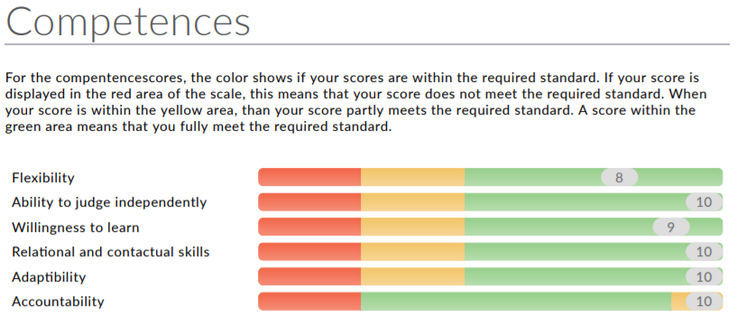
Figures 3.1. and 3.2. show that both Pieter and Joost are a good match with the company with regard to their competencies. Joost scored slightly higher than Pieter for most competencies. However, a high score for the Responsibility competency is not necessarily positive. In general, the test showed that both Pieter and Joost had sufficient competencies required for this job and that they could cope well with the challenges it entails.
During a follow-up interview, both men said that they could recognise themselves in their scores. Pieter said that he had regularly approached his previous employers with suggestions during a project. He sometimes thought that it was a pity that he was only expected to follow instructions, even though he wanted to contribute ideas to improve operations. This is in line with his high scores for ‘independent judgement’ and ‘responsibility’.
Joost was somewhat surprised by his high scores for the competencies, especially the fact that his high score for responsibility fell in the yellow part of the graph. During his follow-up interview, several stories emerged that that made his scores more plausible for him. For example, during his study, he had often taken the lead during group projects. Although he enjoyed this leadership role, it was sometimes difficult for him to let the other group members do their thing. He was very keen to get a good result and was inclined to check everything or to take everything upon himself. This pitfall made the score for ‘responsibility’ recognisable after all.
Figure 3.3. Pieter’s skills
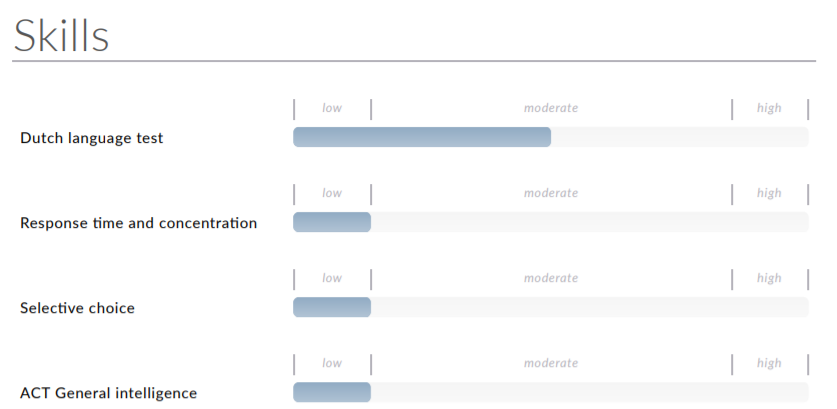
Figure 3.4. Joost’s skills

If we look at the different skills in Figures 3.3. and 3.4, we do not initially see many differences between the two candidates. Their scores for the Dutch language test were virtually identical. Their language level is therefore sufficient for them to be able to cope with the training course and the job.
Neither candidate scored very highly for a simple reaction time task. Pieter’s score was on the border between a pass and a fail, while Joost’s score was just above this line.
The more detailed results (not shown here) show that both men had an average reaction speed time, but that they made quite a lot of mistakes. This means that they often reacted too soon or failed to see a stimulus in time. In other words, both candidates responded normally when they recognised a stimulus, but they often failed to see one or thought that they had seen one when they had not.
Joost scored higher than Pieter for the selective choice reaction time test. Pieter also made quite a lot of mistakes in this. His performance, however, was more stable than that of Joost, whose reaction times fluctuated, although they were good on average.
The main difference between the two candidates emerged when we looked at ACT General Intelligence. Once more, Pieter’s score hovered around the pass/fail line, while Joost’s score was more than adequate.
Pieter’s score was below average when compared to the education level 4: post-secondary education norm group, while Joost’s score was average for this norm group. As the minimum cognitive and work level required of candidates was education level 4: post-secondary education, Pieter’s score was too low.
Figure 3.5. Details ACT General Intelligence Pieter

Figure 3.6. Details ACT General Intelligence Joost

If we look at the scores per sub-test (Figures 3.5. and 3.6.), we can see that the score for the Figure Sets test, which measures abstract reasoning abilities, is approximately the same for both candidates. They both scored in line with the expectations for someone who can think and work at education level 4: post-secondary education level. This sub-test is the clearest measure of a person’s fluid intelligence. Although the Digit Sets sub-test also primarily measures fluid intelligence it is assumed that people taking this sub-test have some basic knowledge of maths.
If we look at Pieter’s scores, we see that he scored considerably lower for the Digit Sets sub-test than for the Figure Sets sub-test. This type of difference may occur in practice. Previous studies show that ACT General Intelligence’s sub-scales have a correlation of approximately .60 (see Chapter 6). In general, we see that someone with high scores for one sub-test also has high scores for the others. However, there are candidates like Pieter who score higher or lower for one particular sub-test. There are different explanations for this, such as a lack of basic skills or dyscalculia.
These types of differences and their possible causes can be discussed with the candidate during the follow-up interview. To interpret the scores, it is particularly important to look at their general trend. In Pieter’s case, we see he had an average score for one sub-test and below average scores for the other two sub-tests. It is easier to interpret Joost’s scores as he had a relatively stable score pattern, where all the scores were around average.
Pieter’s scores for the Verbal Analogies sub-test was also below average. It is assumed that Verbal Analogies requires the most prior knowledge of all the sub-tests. This does not mean, however, that this test only measures crystallized intelligence. The items have been designed so that most people taking the test will know the words used in it. The difficulty of the items lies mainly in discovering more complex relationships and patterns. We cannot therefore jump to the conclusion that a lower score for this specific sub-test indicates a lower language level.
This is also illustrated by this case. Although Pieter’s score for the Dutch language test was sufficient, his score for Verbal Analogies was below average. Joost’s score for the Dutch language test was similar to Pieter’s, but his score for Verbal Analogies was average. From this, we can conclude that Pieter’s below average score was mainly a reflection of his verbal reasoning abilities and that his language level cannot fully explain this below-average score.
During the follow-up interview, Pieter expressed disappointment with his scores. He said that he had been very nervous about the assessment day. At school and college he had found written texts very difficult and had always been nervous of them, despite doing well in practical tests. He described himself as a ‘practical man’. The only explanation he could give for his low Digit Sets score was that mathematics had always been one of his worst subjects at school.
Joost was satisfied with his scores, and had had a good feeling about the tests during his assessment day. The only thing that disappointed him slightly was his scores for the reaction time tests. He explained this by saying that they were the last tests of the day and that the day had been longer than he expected. As he had an appointment that evening, he was worried about getting home on time and noticed that he had difficulty concentrating.
Conclusion
Even though his personality suited the job, Pieter was turned down. His reaction time scores contained too many errors, something that could lead to dangerous situations. ACT General Intelligence also showed that he could not think or work at education level 4: post-secondary education. This meant that there was a risk that the training course would be too difficult for him, causing him to drop out early.
Joost was accepted as a driver. His performance for the reaction time and concentration test was rather low, but still sufficient. His ACT General Intelligence scores showed that he had sufficient cognitive abilities to be able to complete the training course successfully.
3.6.3.2. Case study on career adviceIntroduction
To give insight into the interpretation of ACT General Intelligence’s test results, we will now discuss case 2, which concerns career advice. In practice, career advice often involves using ACT General Intelligence together with the Work-related Personality Inventory, Work Values and Questionnaire for Interest in Tasks and Sectors, in order to gain a picture of a person’s personality traits, motivations and interests. Depending on the research question, ACT General Intelligence can be used separately or in combination with these questionnaires.
A brief description of the situation
Pim Kuijpers is a young man, aged 23. In his last year of primary school, he was advised to follow education level 2: lower secondary education, where he followed the theoretical track. Throughout his first year, he struggled with this new way of learning: he had difficulty with having to learn several different subjects and the test weeks at the end of each period. However, he felt that education level 2: lower secondary education was the right place for him, and he discovered an interest in economics. He was motivated and after obtaining his education level 2 certificate with an average score of 7.3, he progressed onwards to class 4 of HAVO, a higher track of secondary education). He soon found himself struggling to learn the vast amounts of exam material and keep up with his homework. After six months of this, he was overstressed and unable to complete the school year. In 2013, he started an education level 4: post-secondary education programme in Financial Services. After completing this programme, he found a graduate internship with an insurance company. He was currently working for the same company as a financial services provider.
Question
Pim noticed that his work was becoming less challenging and that he wanted to continue his studies so that he could gain promotion within the company, and maybe work as a financial advisor. He was considering following an education level 6: bachelor or equivalent programme in Financial Service Provision, but was wondering whether this would be a wise choice and if he was capable of doing it.
He took the following tests and questionnaires to find an answer to his question.
- Work-related Personality Inventory - Normative (WPIN)
- Career Values - Ipsative (CVI)
- Interest Questionnaire for Tasks and Sectors (ITS)
- ACT General Intelligence
Test result
ACT General Intelligence
ACT General Intelligence was used to determine Pim’s general intelligence. The results are shown in Figure 3.
Figure 3.7. Results of Pim’s ACT General Intelligence


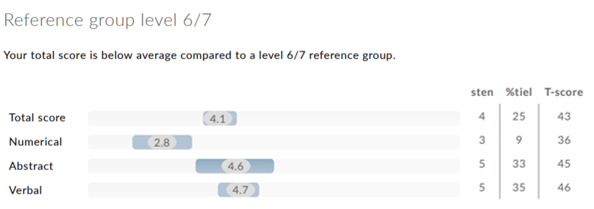
ACT General Intelligence gives an indication of a person’s IQ score with a confidence interval per sub-test and a total. In the current case study, the sten score was requested in comparison with the reference group for education level 4: post-secondary education and education level 6: bachelor or equivalent.
The IQ score as a general measure of intelligence states an average score (100) to indicate average intelligence. If we look at the IQ score per sub-test for the Abstract sub-test (Figure Sets) and the verbal sub-test (Verbal Analogies) we see that the scores also indicate an average abstract and verbal cognitive ability. The numerical sub-test (Digit Sets) in relation to the other sub-tests shows that the candidate’s numerical analytical abilities are weaker than his abstract and verbal cognitive abilities. The IQ score for the numerical sub-test is slightly below average.
If the scores are compared with the education level 4: post-secondary education reference group, the total score is around average. This means that Pim’s general intelligence corresponds with an education level 4: post-secondary education thinking level. It is clear that Pim’s scores for abstract and verbal reasoning abilities are average and his numerical scores are below average. In comparison to the education level 6: bachelor or equivalent norm group, his general intelligence is below average. In comparison to the education level 6: bachelor or equivalent norm group, Pim scored just below average for abstract and verbal reasoning abilities, while his numerical reasoning abilities were well below average.
In the interview, Pim said that this was confronting, but recognisable. He said that he could manage education level 4: post-secondary education perfectly well, but had had to work extremely hard to keep up when he attempted to follow a higher stream of secondary education (HAVO). Pim also said that he had really struggled with the numerical sub-test but had found the verbal sub-test easier.
In short, ACT General Intelligence revealed that Pim seems to have an average degree of intelligence. Compared with education level 6: bachelor or equivalent and the education level 4: post-secondary education reference groups, ACT General Intelligence indicates that Pim’s thinking abilities are education level 4: post-secondary education, whereby his conceptual and verbal abilities are stronger than his numerical abilities.
Personality
The Work-related Personality Inventory reports on five factors, each of which contains a number of scales (see Figure 3.8.).
Figure 3.8. Results of Pim’s WPIN

If we look at the complete personality profile, it shows a varied score profile with some clearly distinct scores and some less distinct scores. The score for the Influence factor (3) is below average, mainly due to a low score for Status (2) and Self-presentation (2). Occupying a high position and drawing attention to himself are personality traits that are less pronounced in Pim. The lower score for Sociability (3) is mainly due to below average scores for Need for contact (3), Socially at ease (3) and Self-disclosure (3). This indicates less need for contact, shyness in social situations and reserve when it comes to sharing one’s feelings. We also see a high score for Structure (8) which means that Pim is quite orderly and structured, whereby Precision (10) in particular appears to be a dominant personality trait. Regularity (8) reveals a preference for rules and procedures. Enthusiasm (5) is average with around average scores for Energy (6), Personal Growth (4), Perseverance (6), Originality (4) and Independence (6). This indicates an average amount of energy and perseverance. Pim is less able to adapt to changes, which can be seen in his score for Innovation (3). The score for emotional stability is in the upper reaches of average (Stability (6)). He has an average degree of Self-confidence (5) and Optimism (5). The most prominent trait is that he can deal easily with criticism (Resilience (8)) and is patient (Frustration tolerance (7)).
Figure 3.9. Results of Pim’s Competencies Indicator
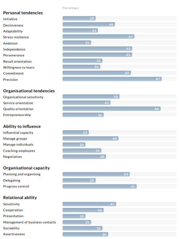
When we look at the personality profile, we see that quality-focus and precision come to the fore as competencies that could easily be developed. To a lesser extent Pim’s talents also lie in progress control, stress-resistance, independence, perseverance, effort, planning and organisation.
Pim generally recognised himself in this personality profile. At his performance review, he had received comments on his emphasis on quality and his precise way of working. He also thinks that these are clear personality traits. At work, he enjoys doing his job according to the regulations and has difficulty with new working methods when they are first introduced. He had expected a higher score for perseverance. He said that he had stayed at the higher track in secondary education until he could no longer continue.
Career values
The career values inventory establishes primary motivators (the most important career values), secondary motivators, neutral motivators and demotivating factors (career values that demotivate). They can be included in a report or read from the graph of the work values that are clustered around Yields, Activities and Environment (see Figure 3.10).
Figure 3.10. Results of Pim’s Career Value Inventory.

There appears to be a balance between the energy that he derives from his private life and his work. The most important career values for Pim are Dynamism (8) and Quality (8). In his current job, this dynamism can be seen in the diversity of client assignments and is important for delivering quality. Financial reward (7), Autonomy (7) Security and Stability (7), Concrete results (6), Career (6) and Enterprise (6) were also important to Pim. He acknowledges that he likes to know where he stands and currently has a well-defined package of tasks and clear agreements on which tasks must be done and when. Pim wanted more autonomy and personal responsibility than he had in his current position. He also wanted to advance in his career. He saw studying further as a way to advance in his career. Demotivating factors are Cooperation (4), Challenging tasks (4), Influencing (4), Creative thinking (4), Praise and recognition (4) and Developing (3). Pim does not really feel the need to exert influence within the team, he prefers it if everyone is allocated their own client assignments and performs his or her own tasks. The opportunity to develop further or do new tasks is not important for Pim.
Interest Questionnaire for Tasks and Sectors
This questionnaire gives a graphic and textual representation of the interest areas, interest in sectors and tasks ranked from high to low. See Figure 3.11.
Figure 3.11. Results of Pim’s ITS

The ITS mainly reveals an interest in the Administration (7) and Commercial services (6) sectors. Pim has a clear preference for these sectors and is distinctly less interested in other sectors, such as Welfare, Safety, Law and Education, training and instruction. This interest matches his current profession, which is at the intersection of these sectors. Other professional and training opportunities within these sectors could be explored.
The tasks that Pim enjoys are found in different task areas. The tasks that interest him most are Maths (5) and Working with computers (5). They are followed by Being Creative (3) and a number of supportive tasks, such as Administrative tasks (4) and Work planning (4). He is interested to a lesser extent in the social tasks that are part of commercial service provision: Assisting (4), Consulting with colleagues (4), Coaching people (4), Convincing people (4) and Maintaining contact (4). These tasks fit with his current job.
He has been drawn to working in commercial services since graduation. He chose his study programme because he was interested in working for a commercial company, even though he knew that he was not suited to working as a sales person. At work, he recognises that he enjoys assessing damage claims, and calculating specific remunerations. At school, he enjoyed economics and doing calculations. He does not recognise being creative, he helps his department by thinking along to solve any problems that may arise with clients but does not really have to be creative at work. He enjoys working for clients, but prefers to have more indirect contact with them.
Conclusion and recommendations
To sum up, Pim is an orderly and well-structured person. He has a good eye for detail and likes to follow rules and procedures. He is patient, can easily deal with criticism and is somewhat reserved and shy when it comes to social contact. He appears to have a reasonable degree of perseverance, energy and self-confidence, which would help him to make the effort needed to follow a level 6: bachelor or equivalent programme. The Financial Service Provision study programme corresponds with his interests and the field in which he works and wants to develop professionally. He appears to think at education level 4: post-secondary education level, which means that his cognitive level is less of a match with the level required by a level 6: bachelor or equivalent programme. A level 6: bachelor or equivalent programme would demand a great deal of extra effort from him and is therefore less suitable. His current job is structured and emphasises quality; this is a good match, both with what Pim wants in a job as well as his focus on quality. Growing within his company would give him the opportunity to bring his job closer to the other career values that are important to him, such as working on his career, more autonomy and personal responsibility.
The recommendation on the basis of these results is that a level 6: bachelor or equivalent programme is less suitable and that Pim should explore opportunities for growth within his company or the financial services sector.
Pim found it difficult to discuss the recommendation. He sees that the level could be too high, also because he had tried to follow a higher track in secondary school and found out that no matter how hard he worked, it never seemed to be enough. It is still difficult for him to accept this.
Epilogue
Pim gave up his job and started a level 6: bachelor or equivalent programme in Financial Services in September. After a few months, he stopped his studies after consulting the student advisor and returned to his employer.
3.6.4. Relevant information for interpreting results
Selection procedures are always stressful for candidates: some can cope well with the tension this entails, while others struggle to deal with it. This may cause some people to perform less well than expected. For instance, a person may suffer from fear of failure or encounter technical problems with the computer when taking the test that will influence the test scores. To gain insight into these types of circumstances, we believe that tests can never be interpreted without an interview. The value of this test mainly lies in the fact that it is fast and gives a broad overview of a person’s personality in work situations. This backs up interviews and meetings with candidates. It is therefore important that when selecting job applicants or making recommendations, that you do not rely solely on the test scores, but also use other sources of information, such as an interview or additional tests, such as tests that measure career values and/or interests.
Furthermore, when interpreting results, it is important to take any background variables that may have influenced the test scores into account. People may show differences in their test scores on the basis of their gender, age, education level or ethnic background, that have little to do with their intelligence. We see this to a small extent in ACT General Intelligence (see Chapter 6). For example, as observed in the literature and many other intelligence tests (see, for example Van den Berg & Bleichrodt, 2000 and Van de Vijver, Bochhah, Kort & Seddik, 2001), we also see that candidates with a migrant background obtain lower scores than candidates with a non-migrant background. Studies conducted into these relationships will be comprehensively described in Chapter 6. These studies conclude that the differences in terms of effect sizes were relatively small, which means that one can take differences into account on the basis of background characteristics, but that this is not strictly necessary for a correct interpretation (see Chapter 4 for a detailed discussion).
3.7. Software and support
The ACT General Intelligence test can be taken on any computer with an internet connection and functioning browser. It does not require the installation of any specific software.
The portal supports all commonly-used desktop internet browsers, such as Microsoft Edge and recent versions of Chrome, Firefox and Safari in Windows XP (and higher), Apple OSX 10.4 or higher and conventional Linux versions. It is possible to take the test on an iPad; however, we do not recommend this as selecting answers (by ticking with your fingers) is more difficult than clicking with the mouse and this can cause problems for some candidates. In view of the large differences between tablets from different brands with regard to specifications and screen resolutions, we cannot guarantee that ACT General Intelligence works on every brand of tablet and therefore we do not recommend using one. The same applies to smart phones. As it is best to take tests for selection procedures in a quiet environment, we recommend taking ACT General Intelligence on a computer or laptop.
In practice, security settings or proxies should not be a problem, provided that they are not too strict. The system does not have high technical requirements, so that it nearly always works in browsers that are not officially supported.
An internet connection is required to take the test in the online system. If the internet connection is lost for a short period while taking the test, answers already given will be saved. If internet access is disrupted for longer, the standard ‘no internet’ report from the browser will be shown. After logging in again, the candidate can continue with the test, but it will start with the next assignment. If this happens, we advise candidates to contact their coach or consultant. Practical experience has shown that this never or hardly ever occurs.
Candidates can contact Ixly’s help desk with questions about system requirements and technical support. The help desk is open every work day from 08.00 to 17.30 via helpdesk@ixly.nl or 088-4959000.
For an overview of frequently asked questions concerning the use of the test portal, please see Appendix 3.2. Appendix 2.1. contains a guide for operating the software. There is more information on operating the test portal at http://www.ixly.nl/kennisbank/test-toolkit-tutorial/ and http://www.ixly.nl/kennisbank/test-toolkit-faq/.
4. Norms
ACT General Intelligence involves norm-focussed interpretation, whereby candidates’ scores are compared with those of a specific norm population. Norm populations in ACT General Intelligence are a representation of four education levels: education level 2: lower secondary education; education level 3: upper secondary education; education level 6: bachelor or equivalent and education level 7: master or equivalent. Weighting ensures that the norm groups correspond in terms of age and gender with persons from the same education levels in the Netherlands. To calculate IQ scores, we also take a norm group that is representative of the working population with respect to education level, age and gender. These distributions are based on data from Statistics Netherlands (CBS) in 2015. This chapter provides a detailed description of how this norm-reference process is conducted and the way in which norm groups are established.
4.1. Norm-reference research
Objective of norm-reference research
ACT General Intelligence was primarily developed for use in selection procedures. It is known that certain aspects of situations may influence tests scores (also see Chapter 2, section 2.4.2 on this). For example, scores obtained in ‘low-stakes’ situations (such as advisory situations intended to give the person taking the test insight into their behaviour without any consequences being attached to the results) may differ from scores obtained in ‘high-stakes’ situations. Selection procedures fall under ‘high-stakes’ situations as there are direct consequences attached to the test scores, such as whether or not your job application is successful. In view of ACT General Intelligence’s user objective we decided to base norm groups on data obtained in real-life selection situations.
We chose to create different norm groups for different education levels. Education level shows a very strong relation with intelligence (see, for example Strenze, 2007) and this is backed up by ACT General Intelligence (see Chapter 6). This means that it would be ‘unfair’, for example, to compare the ACT General Intelligence scores of someone with education level 2: lower secondary education with those of someone with education level 7: master or equivalent. ACT General Intelligence is also intended for selection purposes: organisations nearly always want candidates with a specific level of education for a job. Job profiles nearly always state the education level required for that position. In practice, it is therefore useful to be able to compare a candidate’s scores with the scores of people with the same education level as the candidate in order to select the best (those with the highest scores relatively).
To create norm groups based on education level, we consulted Ixly’s database. This chapter will look at each norm group separately to see how data were collected and norm groups were established. First, we will provide some general background information on this process.
Other differences between groups
We found a number of significant differences in ACT General Intelligence scores for the background variables of gender, age and ethnicity (migrant/non-migrant background). Research into this will be described in detail in section 6.8 of Chapter 6. This study revealed that the differences found largely corresponded to findings from previous studies described in the literature. There were also significant differences in the background variables in terms of effect size (Cohen, 1988), but not enough to be of major practical relevance. It may be interesting to include these differences in the interpretation, as they often concern actual differences, but this is not strictly necessary (see next section). Unfortunately we have no information on the ethnicity, region and work sector of the candidates who have taken ACT General Intelligence in selection procedures. During the calibration study it was shown that no or only very small differences can be expected with regard to region and work sector in ACT General Intelligence.
Should we have separate norms?
Apart from the size of the anticipated effects, it is also possible to discuss whether or not actual differences should be ‘corrected’ by means of different norm references (Bochhah, Kort, Seddik, & Van de Vijver, 2001; Drenth, 1988; Tellegen, 2000; Van den Berg & Bleichrodt, 2000). The considerations that may play a role here can best be clarified by means of an example. Let’s take the example of a coach of a mixed korfball team who selects players according to height, as they know that their team has a better chance of winning with taller players. Say that men are on average 15 cm taller than women. There are two people eligible for selection for the team: a woman who is 1.80 m tall and a man who is 1.85 m tall. As women are smaller on average, the woman will score above average with regard to height in comparison with other women (e.g. a sten score of 8). The man, in contrast, will be average in comparison with other men (e.g. a sten score of 5). Therefore, if there were separate norm groups for men and women regarding height, the coach would select the woman on the basis of the norm-referenced scores. However, compared with the total population (men and women together) the man will have a higher norm-referenced score (i.e. in comparison with the norm population). As he is taller, he is more likely to perform better than the woman. In other words, the coach wants the tallest korfball player in comparison with the population, not the tallest male korfball player compared with other male korfball players or the tallest female korfball player compared with other female korfball players. If different standards apply to people from different groups, these people can no longer be compared with each other (Tellegen, 2000).
This example also applies to ACT General Intelligence; previous research, for example, has shown that fluid intelligence slowly declines with age from adolescence onwards (see, for example, Kaufman & Horn, 1996). However, it is not desirable to ‘normalise' these real differences away: once more, an organisation will most likely want to hire the person with the highest intelligence level (compared to other people with his or her level of education), not the person with the highest intelligence level compared to other people of his or her age. The same applies to gender, although the differences found in ACT General Intelligence are so slight that they have no practical relevance anyway (see Chapter 6).
Naturally, the coach may want an equal distribution of men and women in their team; in that case there are other, very different considerations involved (namely diversity) than just profit or performance maximisation. In real life, selection is ultimately a policy decision on how to strike a balance between 'equal opportunities' and 'efficiency' under the circumstances and given the economic and political preconditions (Drenth, 1988).
This example makes it clear that one must never lose sight of the purpose for which a test is being used. Someone, for example, who has moved to the Netherlands from abroad for work must be compared to the Dutch working population (as opposed to the working population in their country of origin) as they will have to work and perform in the Dutch labour market. Naturally, they must have sufficient command of the Dutch language (if the test is taken in Dutch) or, if the test is taken in the language of their country of origin, the measurement invariance of the translated test must have been sufficiently demonstrated, in order to avoid distortions of the test scores.
We therefore subscribe to the recommendation (Ter Laak & Van Luijk, as cited in Bochhah, Kort, Seddik, & Van de Vijver, 2001) that people from different groups can be compared accurately with the ‘general’ norm population as long as one does not lose sight of the fact that their background, characteristics and specific features can be important – either at an early stage of the selection process, during interpretation of and feedback on the test scores and/or during the interview. For example, when interpreting the test scores of a candidate with a migrant background, their individual background, such as how long they have lived in their new country, their ethnic background and language proficiency level, may all be taken into account (Van den Berg & Bleichrodt, 2000). The data described in Chapter 6, section 6.8.4 may be helpful in this respect. For example, if a candidate with a migrant background has a relatively low, deviating score for Verbal Analogies even though they have scored relatively better for Digit Sets and Figure Sets, you could discuss the possible causes with them; for example, Dutch might not be spoken in their home. It is also possible to compare persons with a migrant background with the general norm table and then select the best within the group of persons with a migrant background or those who score above a certain minimum (Te Nijenhuis & Evers, 2000).
For the reasons set out above we do not use separate norm groups based on gender, region, age or ethnicity.
General comments on norm-reference research
The data were collected from a large number of organisations, spread throughout the country and from all kinds of sectors. These data were collected for the selection of personnel in (among others) the (online) retail sector, health organisations, finance, purchasing, business intelligence, logistics, aviation, transport, technology/industry, healthcare, education, the media sector and the public sector. Among Ixly’s clients are selection and assessment agencies, who use ACT General Intelligence for diverse clients from a wide range of sectors. With regard to the variety of jobs and sectors, we may therefore expect that the results collected for ACT General Intelligence are sufficiently diverse.
The analyses from the other chapters in this guidebook were conducted between July and December 2016, and are therefore based on data up to and including July 2016. Because the norm groups for education level 2: lower secondary education, education level 6: bachelor or equivalent and education level 7: master or equivalent were relatively small on the basis of this data and there was not enough diversity in the education level 3: upper secondary education group, new data obtained in selection situations and collected between July 2016 and December 2016 were added to the norm groups.
The test scores could be distorted if they were mainly collected from a single customer because, for example, this customer would only use tests for applications within a certain sector. That is why we have tried to use as many data sources as possible for the norm groups and have collected norm data from as many different customers and companies from different sectors as possible. One goal was that no more than 20% of candidates within a specific norm group could come from one data source. This largely succeeded, with the exception of the education level 2: lower secondary education group: therefore this norm group must be considered as a provisional norm group. This is explained in more detail below. The representativeness of the norm groups will also be discussed. In line with Cotan’s (2009) guidelines, the maximum weighting factors for representativeness on the gender and age variables in all the cases did not exceed 2, unless stated otherwise.
4.2. Description of the norm groups
Table 4.1. and 4.2. show the characteristics of the norm groups before and after weighting and the distribution of the background characteristics in the norm populations as obtained from Statistics Netherlands. Below is a description of the relevant characteristics for each norm group. When qualifying the size of the correlations between ACT General Intelligence scores and gender/age we used Cohen’s (1988, 1992) guidelines: <.10: trivial, .10 - .30: small to average, .30 - .50: average to large, >.50: large to very large.
|
Table 4.1. Distributions for age and gender in education level 2: lower secondary education and education level 3: upper secondary education. |
|||||||
|
Level 2 |
Level 3 |
||||||
|
Research group (N = 321) |
Weighted norm group (N = 300) |
Statistics Netherlands 2015 % |
Research group (N = 659) |
Weighted norm group (N = 659) |
Statistics Netherlands 2015 % |
||
|
Gender: |
|||||||
|
Male |
252 (78.5) |
183 (61.0) |
55.7 |
349 (53.0) |
358 (54.3) |
53.1 |
|
|
Female |
69 (21.5) |
117 (39.0) |
44.3 |
310 (47.0) |
301 (45.7) |
46.9 |
|
|
Age: |
|||||||
|
15-24 |
62 (19.3) |
90 (30.0) |
30.5 |
60 (9.1) |
114 (17.4) |
17.4 |
|
|
25-44 |
179 (55.8) |
96 (32.0) |
26.0 |
310 (47.0) |
268 (40.7) |
40.7 |
|
|
45-65 |
80 (24.9) |
114 (38.0) |
43.5 |
289 (43.9) |
277 (42.0) |
42.0 |
|
Education level 2: lower secondary education
In total, we obtained test scores from 321 people at education level 2: lower secondary education between July 2015 and December 2016. 74% of the data for this group were obtained from a single client from the transport sector. The remaining data were obtained from 21 other data sources. This gave an uneven distribution with regard to males and females in the research group: in total, 78.5% were male (Table 4.1.). Distribution according to age in the three age categories 15-25, 26-45 and 46-65 also deviated strongly from the distribution in the norm population. We tried to correct this distortion by means of weighting. A second objective was to keep the norm group as large as possible. Eventually the weighting led to the distribution regarding age and gender shown in Table 4.1. After weighting, the distribution for gender (χ2(1) = 3.39, p = .07) did not differ significantly from the respective distribution in the norm population. The age distribution scarcely differed from the age distribution in the norm population (χ2(2) = 6.28, p = .04, V = .10). Unfortunately it was not possible to comply with the set requirement (Cotan, 2009) that the maximum weighting <2 (the maximum weighting was 2.32). Furthermore, due to weighting, the weighted N became 300 (compared to an unweighted N of 321).
The average age in the weighted education level 2: lower secondary education norm group was 37.5 (SD = 13.8, Min.-Max = 17-63). The women (M = 46.9, SD = 14.0) were significantly and considerably older than the men (M = 31.5, SD = 10.4) in this sample (F(1,297) = 124.8, p = .00, Cohen’s d = -1.25). Women scored significantly lower than men for Digit Sets, Figure Sets and the g score, although the effect sizes indicated small to average differences (respectively r = -.25, -.30, -.24). The same applied to negative effects found for age on the g score and scores for Digit Sets and Figure Sets (respectively r = -.15, -.15, -.31). A linear regression also showed that the effect of age disappeared for Digit Sets (B = -.001, p = .84) and the g score (B = -.001, p = .65) when controlled for gender.
In view of the fact that much of the data came from a single source and that the maximum weighting was >2, this norm group must be regarded as being provisional. However, given the score distribution (Table 4.3.), this group seems to be a reasonable representation of persons with education level 2: lower secondary education in the Dutch working population.
Education level 3: upper secondary education
In total, we obtained ACT General Intelligence test scores from 1213 people, collected between July 2015 and December 2016. In this group also, a large proportion of the data had been obtained from the same source that had provided the data for the education level 2: lower secondary education group (685 people; 56.5%). In order to guarantee the representativeness of the norm group, a random sample was taken from these 685 people, which ended up in the final norm group. The number of persons drawn from this specific group was determined by the requirement that no more than 20% of the final norm group should be collected from one data source. This means that 131 people were randomly selected from this group. In total, the data were collected from 66 data sources. Three of the sources contributed a fairly large share of candidates (two contributed 20% and one contributed 15%), but in general each data source only contributed a small number of candidates. The average percentage obtained from a data source was 1.5% (median was 0.3%). This ensures that not one single data source is over-represented in this norm group and that there is a wide range of candidates from different sectors.
The final norm group consisted of 659 people. The gender distribution was almost identical to the distribution in the norm population (χ2 = .00, p = .95), while proportionally there were slightly too few young people in the sample and too many people between 25 and 45 years of age (χ2(2) = 33.04, p = .00). Weighting was used to ensure that age distribution was representative of the norm population. After weighting, the distribution for gender was still representative (χ2(1) = 0.41, p = .53).
The average age in the weighted education level 3: upper secondary education norm group was 40.1 (SD = 12.3, Min.-Max = 19-64). Although the women (M = 42.8, SD = 11) were significantly older than the men (M = 37.9, SD = 10.4) in this sample (F(1,297) = 27.7, p = .00) this difference was not too large (d = -.41). The negative correlations with gender (women scored lower than men in all parts of ACT General Intelligence in this norm group; r = -.29, -.15, -13 and -.25 for Digit Sets, Figure Sets, Verbal Analogies and the g score respectively) and age (r = -.15, -.24 and -.15 for Digit Sets, Figure Sets and the g score respectively) are small to average. No age effect was found for Verbal Analogies.
|
Table 4.2. Distributions for age and gender in education level 6: bachelor or equivalent and education level 7: master or equivalent. |
|||||||
|
Level 6 |
Level 7 |
||||||
|
Research group (N = 570) |
Weighted norm group (N = 570) |
Statistics Netherlands 2015 % |
Research group (N = 490) |
Weighted norm group (N = 490) |
Statistics Netherlands 2015 % |
||
|
Gender: |
|||||||
|
Male |
314 (55.1) |
287 (50.3) |
50.3 |
258 (52.7) |
272 (55.5) |
52.8 |
|
|
Female |
256 (44.9) |
283 (47.6) |
47.6 |
232 (47.3) |
218 (44.5) |
47.2 |
|
|
Age: |
|||||||
|
15-24 |
40 (7.0) |
41 (7.2) |
7.0 |
75 (15.3) |
11 (2.3) |
2.3 |
|
|
25-44 |
315 (55.3) |
315 (55.3) |
53.5 |
317 (64.7) |
278 (56.7) |
56.7 |
|
|
45-65 |
215 (37.7) |
214 (37.5) |
39.5 |
98 (20.0) |
201 (41.0) |
41.0 |
|
Education level 6: bachelor or equivalent
Data was collected from a total of 570 candidates provided by 67 data sources (between July 2015 and December 2016), whereby a maximum of approximately 20% was provided by one data source. The average percentage of candidates per source was 1.5% (median 0.4%).
In terms of representativeness with regard to gender, men were slightly overrepresented in the sample (χ2(1) = 5.30, p = .02). The sample was representative with regard to the three age categories in comparison with the norm population (χ2(2) = .76, p = .68). Weighting ensured that the norm group was fully representative for gender. The weighted norm group was representative with regard to age (χ2(2) = .88, p = .64).
The average age in the weighted education level 6: bachelor or equivalent norm group was 39.8 years of age (SD = 11.2, Min.-Max = 18-67). The women (M = 40.9, SD = 10.6) were slightly younger than the men (M = 38.8, SD = 11) in this sample (F(1,568) = 4.6, p = .03) but this difference was small (d = .18). No effect was found for age and gender in the Verbal Analogies sub-test. The other negative correlations with age (r = -.19, -.31, and -.22 for Digit Sets, Figure Sets and the g score respectively) and gender (women scored lower than men r = -.16, -.14 and -.12 for Digit Sets, Figure Sets and the g score respectively) are small to average.
Education level 7: master or equivalent
In total, we obtained test scores from 490 candidates with education level 7: master or equivalent, collected between July 2015 and December 2016. These data were collected from 56 data sources. In the education level 7: master or equivalent group, it was not fully possible to meet the requirement that one source should not contribute too large a share of the norm group as approximately 27% of the candidates in this norm group came from one data source. However, the average percentage of candidates per source was 1.8% (median 0.3%).
The unweighted norm group was representative of the norm population with regard to gender (χ2(2) = .00, p = .95). In terms of age, both younger people and older people were under-represented in the sample (χ2(1) = 418.99, p = .00; see Table 4.2.). Weighting ensured that the final norm group was fully representative for age in comparison with the norm population. After weighting, the sample was still representative for gender (χ2(1) = 1.46, p = .23).
The average age in the weighted education level 7: master or equivalent norm group was 39.2 years of age (SD = 11.3, Min.-Max = 22-62). Men (M = 38.6, SD = 11) did not differ significantly from women (M = 39.9, SD = 10.9) in terms of age (F(1,488) =.29, p = .59). No differences between men and women were found in the Verbal Analogies sub-test. The gender differences for the other parts were small (r = -.12, -.15, -.14 for Digit Sets, Figure Sets and the g score respectively). The negative effect of age on the scores obtained was small to average for Digit Sets (r = -.36) and Verbal Analogies (r = -.23), while for Figure Sets (r = -.46) and the g score (r = -.45) the effect can be classified as average to large.
The correlations between age and the g score and the scores for the Figure Sets sub-test are rather high. These effects are not easy to explain from the literature as studies mainly examine the relationship between age and intelligence in an entire population, not in different levels of education separately.
These effects therefore seem to derive from the specific composition of the norm group. Inspection of this norm group showed that the persons whose scores had been obtained from the largest data source were considerably younger than persons whose scores had been obtained from other organisations (M = 25.6 years, SD = 3.4 in comparison with M = 37.1 years, SD = 10.4, ||d| = 1.49). The lower standard deviation also indicates that this group was extremely homogenous in terms of age. This group also had considerably higher ACT General Intelligence scores than the rest of the norm group (g score: M = 1.17, SD =.40 in comparison to M = .84, SD = .49, ||d|| = .73). This combination of effects seems to be partially responsible for the high correlations between the test scores and age.
Without this specific group, the correlations between Digit Sets, Figure Sets, Verbal Analogies and the g score and age were -.30, -.41, -.18 and -.38 respectively. Although still rather high, these correlations are approaching more acceptable values.
The solution to this seems to lie mainly in collecting more test scores from a range of organisations in order to obtain a more representative picture of the education level 7: master or equivalent group. We will add new test data to the education level 7: master or equivalent norm group as soon as possible in order to remedy the current shortcomings.
Description of scale characteristics in the norm groups
Table 4.3 to Table 4.6 show the characteristics of the raw scores (θ) for ACT General Intelligence scales for the weighted norm groups. This gives users an overview of the distribution of the raw scores in the norm populations.
|
Table 4.3. Characteristics of the raw scores (θ) for ACT General Intelligence for the Level 2 norm group N = 300). |
||||||||||
|
Min. |
Max. |
Average |
SD |
Skewness |
Kurtosis |
|||||
|
Value |
SE |
Value |
SE |
|||||||
|
Digit Sets |
-2.33 |
2.53 |
-.33 |
.64 |
.24 |
.14 |
.58 |
.28 |
||
|
Figure Sets |
-1.90 |
1.91 |
-.23 |
.64 |
.12 |
.14 |
.14 |
.28 |
||
|
Verbal Analogies |
-2.61 |
1.99 |
-.18 |
.75 |
-.35 |
.14 |
.47 |
.28 |
||
|
g score |
-1.97 |
1.29 |
-.24 |
.53 |
-.12 |
.14 |
.12 |
.28 |
||
|
Table 4.4. Characteristics of the raw scores (θ) for ACT General Intelligence for the Level 3 norm group N = 659). |
||||||||||
|
Min. |
Max. |
Average |
SD |
Skewness |
Kurtosis |
|||||
|
Value |
SE |
Value |
SE |
|||||||
|
Digit Sets |
-2.42 |
2.23 |
-.12 |
.70 |
.24 |
.10 |
.52* |
.19 |
||
|
Figure Sets |
-2.19 |
2.42 |
-.06 |
.78 |
.36* |
.10 |
.19 |
.19 |
||
|
Verbal Analogies |
-2.50 |
2.38 |
.05 |
.77 |
-.46* |
.10 |
.18 |
.19 |
||
|
g score |
-2.11 |
1.74 |
-.04 |
.61 |
-.21 |
.10 |
.08 |
.19 |
||
|
Table 4.5. Characteristics of the raw scores (θ) for ACT General Intelligence for the Level 6 norm group N = 570). |
||||||||||
|
Min. |
Max. |
Average |
SD |
Skewness |
Kurtosis |
|||||
|
Value |
SE |
Value |
SE |
|||||||
|
Digit Sets |
-1.77 |
2.58 |
.42 |
.78 |
.31* |
.10 |
.05 |
.20 |
||
|
Figure Sets |
-1.96 |
2.44 |
.42 |
.78 |
.21 |
.10 |
-.44 |
.20 |
||
|
Verbal Analogies |
-1.75 |
2.39 |
.64 |
.66 |
-.53* |
.10 |
1.42* |
.20 |
||
|
g score |
-1.60 |
2.01 |
.50 |
.56 |
-.32* |
.10 |
.56* |
.20 |
||
|
Table 4.6. Characteristics of the raw scores (θ) for ACT General Intelligence for the Level 7 norm group N = 490). |
||||||||||
|
Min. |
Max. |
Average |
SD |
Skewness |
Kurtosis |
|||||
|
Value |
SE |
Value |
SE |
|||||||
|
Digit Sets |
-1.12 |
2.70 |
.77 |
.77 |
.23 |
.11 |
-.25 |
.22 |
||
|
Figure Sets |
-0.97 |
2.46 |
.80 |
.78 |
.04 |
.11 |
-.75* |
.22 |
||
|
Verbal Analogies |
-0.77 |
2.55 |
.94 |
.54 |
.16 |
.11 |
.48 |
.22 |
||
|
g score |
-0.48 |
2.29 |
.83 |
.50 |
-.16 |
.11 |
-.18 |
.22 |
||
An asterisk (*) indicates that the Z score (obtained by dividing the values by their standard error) of skewness and kurtosis (flatness) exceeds the ± 2.58 limit. This threshold value is often used as an indication that a distribution deviates from the theoretical normal distribution. In the education level 2: lower secondary education and education level 7: master or equivalent norm groups, all skewness and kurtosis values lie between - 2.58 and + 2.58. This is not the case for the education level 3: upper secondary education and education level 6: bachelor or equivalent groups. In the education level 3: upper secondary education norm group, the test scores for Figure Sets and Verbal Analogies show relatively skewed distributions, while the distribution of the Digit Sets shows a somewhat larger peak than expected. In the education level 6: bachelor or equivalent norm group, the test scores for Digit Sets, Verbal Analogies and g scores show relatively skewed distributions, while the distribution of the g score and, in particular, Verbal Analogies show a larger peak than expected. However, some people find that the ||Z||>2.58 rule of thumb is extremely strict, and they therefore use more liberal rules in which absolute values of skew > 3 and kurtosis > 8 (or even >10) indicate a deviation from the normal distribution (Kline, 2005). Based on these rules, we can generally conclude that ACT General Intelligence’s test scores are reasonably normally distributed in the four norm groups.
Working population norm group for the IQ score
As ACT General Intelligence also reports IQ scores, whereby ACT General Intelligence scores are not compared to a certain level of education but to the entire population, a norm group that is representative of the entire working population of the Netherlands has also been developed. This norm group is based on the four (unweighted) norm groups plus additional data obtained from persons who took ACT General Intelligence tests in selection situations. Therefore the ACT General Intelligence scores of 2761 people from 111 organisations were collected. The maximum share of one organisation was 39.4% and the average share was 0.9% (median = 0.1%). The distribution according to education level in the total norm group is shown in Table 4.7.
|
Table 4.7. Distribution of education levels in the working population norm group, unweighted. |
||
|
Freq. |
% |
|
|
Primary school/education |
38 |
1.4 |
|
Level 2 |
321 |
11.6 |
|
Level 3 |
1213 |
43.9 |
|
Level 2: upper secondary track |
79 |
2.9 |
|
Level 2: pre-university track |
50 |
1.8 |
|
Level 6 |
570 |
20.6 |
|
Level 7 |
490 |
17.7 |
|
Total |
2642 |
100 |
Table 4.8. shows the characteristics of the working population norm group before and after weighting and the distribution of the background characteristics in the norm population (total working population) obtained from Statistics Netherlands. Men were overrepresented in the unweighted norm group. This also applied to middle-aged people and people with a higher level of education. Older people and people with a lower level of education were underrepresented. As education level shows the strongest relation with ACT General Intelligence scores, it was decided that after weighting the norm group for this background characteristic should be fully representative of the norm population. Therefore, different objectives played a role in the weighting: the weighting factor could not exceed 2, the norm group had to be representative in terms of education level and the weighted norm group had to remain as large as possible. Taken together, these three considerations ultimately resulted in the distribution of gender, age and education shown in the third column of Table 4.8. The weighted norm group differed somewhat from the norm population with regard to gender (χ2(1) = 25.04, p = .00) and age (χ2(2) = 80.09, p = .00), but these differences were relatively small (Cramer’s V was .07 and .12 respectively).
|
Table 4.8. Distributions of gender, age and education in working population |
||||
|
Working population |
||||
|
Research group (N = 2761) |
Weighted norm group (N = 2761) |
Statistics Netherlands 2015 % |
||
|
Gender: |
||||
|
Male |
1793 (64.9) |
1601 (58.0) |
53.2 |
|
|
Female |
968 (35.1) |
1160 (42.0) |
46.8 |
|
|
Age: |
||||
|
15-24 |
359 (13.0) |
500 (18.1) |
16.1 |
|
|
25-44 |
1497 (54.2) |
1408 (51.0) |
42.1 |
|
|
45-65 |
905 (32.8) |
853 (30.9) |
41.8 |
|
|
Education: |
||||
|
Low |
359 (13.0) |
623 (22.6) |
22.6 |
|
|
Mid |
1342 (48.6) |
1180 (42.7) |
42.7 |
|
|
High |
1060 (38.4) |
959 (34.7) |
34.7 |
|
The average age in the weighted norm group was 37.2 years of age (SD = 11.9, Min.-Max = 17-67). Although the women (M = 38.3, SD = 13.3) were significantly older than the men (M = 36.3, SD = 11.0) in this sample (F(1,297) = 18.9, p = .00), this difference was small (d = -.16).
The correlations with gender were only significant for Verbal Analogies and the g score, but small with regard to effect size (r = .10 and r = .05 respectively, with women scoring slightly higher than men). The negative correlations with age were slightly larger, but can still be considered small to average (r = -.18, -.27, -.08 en -.18 respectively for Digit Sets, Figure Sets, Verbal Analogies and the g score).
Table 4.9 shows the characteristics of the raw scores (θ) for ACT General Intelligence scales for the total weighted norm group.
|
Table 4.9. Characteristics of the raw scores (θ) for ACT General Intelligence, working population norm group (N = 2761). |
||||||||||
|
Min. |
Max. |
Average |
SD |
Skewness |
Kurtosis |
|||||
|
Value |
SE |
Value |
SE |
|||||||
|
Digit Sets |
-2.42 |
2.70 |
.10 |
.84 |
.31* |
.05 |
.11 |
.09 |
||
|
Figure Sets |
-2.22 |
2.46 |
.18 |
.85 |
.26* |
.05 |
-.26* |
.09 |
||
|
Verbal Analogies |
-2.76 |
2.55 |
.26 |
.84 |
-.35* |
.05 |
.16 |
.09 |
||
|
g score |
-2.11 |
2.29 |
.18 |
.71 |
-.08 |
.05 |
-.24 |
.09 |
||
Although some Z values of skewness and kurtosis (obtained by dividing them by their standard error) were greater than 2.58, the alternative criteria set by Kline (2005) were amply met. We may therefore conclude that the ACT General Intelligence test scores are fairly normally distributed in the total norm group.
In ACT General Intelligence the raw scores are converted into standardised scores, so that they can be compared with the norm group. These standardised scores will be discussed in the next section (also see Chapter 3).
4.3. Used scores and norm tables
ACT General Intelligence reports on the sten scores, T-scores, percentile scores and IQ scores. In each scale, the raw scale scores are first converted into a Z score and then into the four aforementioned standardised scores. Standard scores give a picture of the way in which a certain score relates to norm populations. In our case this concerns the four education levels mentioned above and the Dutch working population. The exact way in which these scores are obtained and how they should be interpreted is discussed in Chapter 3.
Appendices 4.1. and 4.2. contain the norm tables for the scales. These tables show the sten score, T-score, percentile score and IQ score that accompany each raw score. The confidence interval (belonging to a confidence level of 80%, 90% and 95%) is also given for the sten score. A confidence level of 80% means that if there is a large number of repetitions of the prediction or estimation of score X, 80% of the calculated intervals will contain the unknown value X (Drenth & Sijtsma, 2006).
We chose this interval for the sten score because experience has taught us that most users use the sten scores to review and discuss the scores and because this interval is also given in the report (see Appendix 3.1. for a sample report).
Sten scores are a form of standard scores with an average of 5.5 and a standard deviation of 2. The 80% confidence interval is therefore calculated as follows:
Lower limit of the confidence interval: 5.5 + 2 * (Z - 1.28 * SEM)
Upper limit of the confidence interval: 5.5 + 2 * (Z + 1.28 * SEM)
The Z score is obtained by subtracting the average of the norm group from the raw θ and dividing it by the standard deviation for this norm group:
θ-μ
The value 1.28 corresponds to the 80% confidence interval, the corresponding values for the 90% and 95% confidence intervals are 1.68 and 1.96 respectively. The higher the confidence level, the wider the confidence interval.
In tests based on traditional test theory (as opposed to item response theory on which ACT General Intelligence is based), reliability is a single measure that gives information about the accuracy of the whole scale. In item response theory, the reliability of the measurement depends upon the location on the θ scale (see Chapter 5). This is why Appendices 4.1. and 4.2. show the norm tables based on different SEM sizes. In the first variant in Appendix 4.1. the SEM is calculated on the basis of the entire item bank: i.e. in each sub-test, the information provided by all sub-test items for the values ranging from -2.5 to 2.5 (in steps of 0.1) has been added up, resulting in the total information (TI) per θ value. The SEM was then calculated using formula 1/√TI for each value of θ. The g score’s SEM is calculated by taking the sum of the information values provided by all items (i.e. from all three sub-tests together) at each θ-value, and then calculating the SEM once more using the above formula.
However, this representation is somewhat misleading, because this would be the SEM if a candidate were to be shown all possible items from the item bank. However, candidates taking ACT General Intelligence only answer a small proportion of these items (a minimum of 10 and a maximum of 17 per sub-test). A simulation study was carried out to give a more realistic picture of the SEM and the corresponding confidence intervals that can be expected with ACT General Intelligence. In this study, 500 'persons' - i.e. θs - were generated for each value between -2.5 and 2.5 in increments of 0.1. Therefore, there were 500 'true θs' with a value of -2.5; 500 'true θs' with a value of -2.4; 500 'true θs' with a value of -2.3 et cetera. This resulted in a total N of 25,500. ACT General Intelligence was then simulated for these 25,500 persons. After this, the average SEM was calculated for every 500 candidates with the same true θ, resulting in 51 average SEM values (i.e. for each value between -2.5 and 2.5). Therefore we may expect these SEM values for values across the entire θ scale. These average SEM values were then shown in the norm tables in Appendix 4.2. and used to calculate the confidence intervals.
5. Reliability
5.1. Introduction
A questionnaire’s reliability gives an indication of its accuracy. The term reliability refers to the reproducibility of the results measured. In other words, to what extent do the initial results obtained using a particular instrument correspond with the results obtained a second time (and a third time, etc.), or to what extent do results correspond with a comparable set of items? This chapter describes studies conducted to examine the reliability of ACT General Intelligence.
Chapter 1 should have already made it clear that traditional ideas about reliability do not apply to IRT models: a measurement’s degree of accuracy depends on where on the θ scale the measurement is taken. It can still be useful, however, to have a general measure of reliability. We therefore calculated the empirical reliability (Zimowski, Muraki, Mislevy, & Bock, 2003) for both the total sample and the candidate sample. Empirical reliability is based on the ratio of the error variance to the total variance:

(5.1)
In this formula, (5.1) ρ is reliability, σ2 is the ‘true’ variance and σ2error is the error variance. The error variance can be calculated by taking the square of the SEM calculated for each person in the sample, and then taking its average over the entire sample. The SEM, or standard error, indicates the distribution that can be expected around the estimated θ: the smaller the distribution, the more accurate the measurement. The ‘true’ variance, σ2, is simply the variance of the estimated θs from the sample.
In addition to empirical reliability, we also looked at the average SEM for the total sample and the candidate sample. As indicated above, however, the SEM depends on where on the θ scale the measurement is taken, which is why we also compared the SEMs with θ.
5.2. Reliability
5.2.1. Empirical reliability
Empirical reliability was calculated for the sub-tests in the total sample and the calibration sample. Table 5.1. shows the variances of the θs and their accompanying error variances. As described above, they can be used to calculate empirical reliability, shown in the last column in Table 5.1. Taking the Figure Sets as an example, the θs have a variance of .763 and the error variance is .234. The empirical reliability is therefore .763 / (.763+.234) = .77.
|
Table 5.1. Empirical reliability |
|||||||
|
Total samplea |
Candidate sampleb |
||||||
|
Variance of θ |
Error variance |
ER |
Variance of θ |
Error variance |
ER |
||
|
Digit Sets |
.837 |
.163 |
.84 |
.713 |
.137 |
.84 |
|
|
Figure Sets |
.763 |
0.234 |
.77 |
.720 |
.167 |
.81 |
|
|
Verbal Analogies |
.884 |
.116 |
.88 |
.699 |
.098 |
.88 |
|
|
g score |
.629 |
.064 |
.91 |
.498 |
.041 |
.92 |
|
|
Note: ER = empirical reliability a N = 6277, b N = 2532. |
|||||||
In the total sample, the reliability of the Digit Sets and Verbal Analogies sub-tests is sufficient to more than sufficient when compared to Cotan’s guidelines (2009; < .80 insufficient, .80 ≤ r ≤ .90 sufficient, r ≥ .90 good). The g score’s reliability is good: it should be noted that this is a kind of average measure that may disguise specific reliabilities depending on the θ scale (Brown, 2014). Moreover, the calibration sample (part of the total sample) also included persons who had only answered a very small number of items: by definition, these people will have a higher SEM and this will have influenced the overall measure of reliability (see next section). Reliability will be good for frequently occurring values of θ (approximately between -1 and 1) (see next section and Figure 5.1. and 5.2.).
We must make an important observation with regard to these results: the g score for the total sample already meets Cotan’s (2009) criteria for 'good' reliability (> .90). However, these reliability levels are also based on responses from the calibration sample where respondents received a subset of linear, not adaptive items - i.e. the items were not geared towards their level. Items in an adaptive test are adapted to a person's level. This means that measurements are more accurate (see right-hand side of Table 5.1) and reliability is higher: at .92, we can say that the reliability of the g score in the adaptive test is good. The reliability of the sub-tests was also relatively high (with an average of .84 it was >.80, ‘sufficient’).
The reliability of Figure Sets was just above the threshold of .80 that Cotan (2009) considers ‘sufficient’ for tests on which important decisions are based, such as rejecting or hiring a candidate in selection situations. The scores for the three sub-tests could also be used for this purpose if the situation requires. For example, if candidates are being selected for a job where numerical skills are important, the sub-tests can be used as they are considered ‘sufficiently’ reliable. However, as this is not the same as 'good' reliability, and in view of the measurement goal and practical purpose of ACT General Intelligence (predicting work performance), we recommend that important decisions, such as selecting a candidate for a job, should be based on the g score (see Chapter 1, section 1.3.2.).
5.2.2. SEM values
We also calculated the average SEM values for the two samples. These are shown in Table 5.2. The g score’s SEM is calculated by adding up the information (= 1/SEM2) provided by the three sub-tests and calculating the SEM once more with this (= 1/√Info).
|
Table 5.2. Accuracy of the θ estimate. |
|||
|
Total samplea |
Candidate sampleb |
||
|
Average SEM |
Average SEM |
||
|
Digit Sets |
.39 |
.37 |
|
|
Figure Sets |
.46 |
.41 |
|
|
Verbal Analogies |
.33 |
.31 |
|
|
g score |
.25 |
.20 |
|
|
a N = 6277, b N = 2532. |
|||
In Table 5.2., we see the same pattern as in Table 5.1.: the reliabilities are sufficient to good, whereby Figure Sets has the lowest reliability and Verbal Analogies the highest.
The reliability levels are slightly higher in the candidate sample (as shown by the lower average SEM values). The g score’s reliability is very high with an extremely low average SEM value of .20.
5.2.3. Reliability among different groups
In order to investigate whether ACT General Intlligence measures in a way that is equally reliable for different sub-groups (male/female, persons with a migrant/non-migrant background, low/middle/high educational level, young/middle-aged/older), the reliability for these sub-groups was calculated separately on the basis of the average SEM. Empirical reliability is less useful for individual groups: as the above formula indicates, the variance of the estimated scores plays an important role in the calculation of this reliability. If the error variance is kept constant (σ2error), a smaller variance in the estimated θs (σ2) will automatically result in lower reliability. Because the sub-groups are more homogenous than the total population, the variances of the true scores among them will be automatically lower (a type of restriction of range). Take, for example, the different education levels groups: considering that intelligence is normally distributed over the entire population, the education level 7: master or equivalent group will be at the right side of the distribution, thus limiting this group’s variance. This problem is not found with people who have attained education level 3: upper secondary education, who are in the middle of the distribution. Therefore, only reliabilities values based on the mean SEM values (1-SEM2) are shown in Table 5.3. (total sample) and Table 5.4. (candidate sample).
|
Table 5.3. Accuracy of the θ estimate for gender, age, education level and ethnicity in total sample – average SEM. |
||||||||||
|
Gendera |
Ageb |
Educationc |
Ethnicityd |
|||||||
|
Male |
Female |
Low |
Middle |
High |
Low |
Middle |
High |
Non-migrant background |
Migrant background |
|
|
Digit Sets |
.83 |
.83 |
.84 |
.84 |
.81 |
.86 |
.81 |
.81 |
.83 |
.82 |
|
Figure Sets |
.78 |
.73 |
.76 |
.76 |
.72 |
.77 |
.72 |
.71 |
.70 |
.69 |
|
Verbal Analogies |
.88 |
.88 |
.89 |
.88 |
.87 |
.85 |
.86 |
.86 |
.87 |
.86 |
|
g score |
.91 |
.90 |
.91 |
.91 |
.89 |
.90 |
.89 |
.88 |
.89 |
.89 |
|
a Sub-tests: Nmen = 2461-2591, Nwomen = 2142-2332, g score: Nmen = 3020, Nwomen = 2941. a Sub-tests: Nlow = 477-505, Nmiddle = 1754-1872, Nhigh = 1970-2143, g score: Nlow = 596, Nmiddle = 2207, Nmiddle = 2755. a Sub-tests: Nlow = 723-1027, Nmiddle = 2209-2344, Nhigh = 1328-1479, g score: Nlow = 1286, Nmiddle = 2838, a Sub-tests: Nnon-migrant background = 2275-2550, Nmigrant background = 378-421, g score: Nnon-migrant background = 3474, Nmigrant background = 535. |
||||||||||
|
Table 5.4. Accuracy of the θ estimate for gender, age, education level and ethnicity in candidate sample – average SEM. |
|||||||||||||
|
Gendera |
Ageb |
Educationc |
Ethnicityd |
||||||||||
|
Male |
Female |
Low |
Middle |
High |
Level 2 |
Level 3 |
Level 6 |
Level 7 |
Non-migrant background |
Migrant background |
|||
|
Digit Sets |
.83 |
.84 |
.83 |
.84 |
.79 |
.76 |
.78 |
.80 |
.82 |
.81 |
.81 |
||
|
Figure Sets |
.81 |
.81 |
.82 |
.82 |
.78 |
.75 |
.78 |
.77 |
.77 |
.90 |
.88 |
||
|
Verbal Analogies |
.88 |
.88 |
.90 |
.89 |
.88 |
.87 |
.87 |
.80 |
.75 |
.74 |
.74 |
||
|
g score |
.92 |
.93 |
.93 |
.93 |
.91 |
.89 |
.90 |
.87 |
.87 |
.90 |
.89 |
||
|
nmen = 1463, Nwomen = 771-773. nlow = 260, Nmiddle = 933, Nhigh = 640. c NLevel 2 = 204, NLevel 3 = 1094-1095, NLevel 6 = 402, NLevel 7 = 327. d Nnon-migrant background = 194, Nmigrant background = 90. |
|||||||||||||
There is more information on distribution within the categories in Chapter 6, section 6.8. The differences between men and women with regard to reliability were small in the total sample. It is also important to note that differences between people with a non-migrant background and people with a migrant background were also small. This means that general intelligence and specific aspects of intelligence can be measured equally reliably for both groups using ACT General Intelligence. The same applies to the three age categories.
The differences among education level were slightly larger in the total sample, and particularly noticeable in the Digit Sets and Figure Sets. In both sub-tests, the measurements were more reliable for people with a lower level of education. This result can be explained when we look at Figure 5.1.: we had already concluded that in the item banks for Digit Sets and Figure Sets, the most informative items were to be found around the lower θ values. This means that measurements in the Digit Sets and Figure Sets are more reliable at a lower θ (and therefore lower educational level): there are simply 'better', more informative items at this point, which give more information about a person's intelligence. However, Table 5.4 shows that this does not lead to less accurate estimates of θ for people with higher θs (i.e. who have higher education levels).
It is interesting to note that in the candidate sample, the reliability of the Digit Sets sub-test was slightly higher for people with a higher level of education (education level 7: master or equivalent) than for people with lower levels of education. In the total sample, we did not see any difference for Verbal Analogies according to education, while in the candidate sample, we see that this measurement was more accurate for people with a low education level. Differences between the total sample and the candidate sample may be due to the sampling method (linear versus adaptive), or differences in variances of the groups studied.
Scarcely any differences in the reliability of the g scores were found in the total sample. The same applies to the candidate sample (consisting of people who had completed the fully adaptive ACT General Intelligence).
5.2.4. Reliability among norm groups
Table 5.5 shows the reliability levels of the ACT General Intelligence norm groups (see the chapter on Norms).
|
Table 5.5. Accuracy of the θ estimate among the norm groups for Level 2, Level 3, Level 6, Level 7 and the Working Population. |
|||||
|
Level 2 |
Level 3 |
Level 6 |
Level 7 |
Working population |
|
|
Digit Sets |
.76 |
.78 |
.81 |
.81 |
.84 |
|
Figure Sets |
.73 |
.79 |
.78 |
.77 |
.82 |
|
Verbal Analogies |
.88 |
.87 |
.81 |
.73 |
.89 |
|
g score |
.89 |
.91 |
.88 |
.85 |
.93 |
|
c NLevel 2 = 300, NLevel 3 = 659, NLevel 6 = 570, NLevel 7 = 490, NWorking population = 2761. |
|||||
As we have said earlier, we recommend that important decisions, such as candidate selection, should be based on the g scores, and that the sub-tests should be primarily used to provide more in-depth clarification. Compared to the guidelines used by Cotan for tests on which important decisions are based (< .80 insufficient, .80 ≤ r ≤ .90 sufficient, r ≥ .90 good), the above data for education level 2: lower secondary education and education level 6: bachelor or equivalent can be considered 'sufficient' (the values are close to .90), the scores for education level 3: upper secondary education and the working population are 'good', while the score for education level 7: master or equivalent is 'sufficient'.
5.2.5. SEM values depending upon the θ scale
As described above, the measures discussed here involve a kind of average measure of reliability, which does not do justice to one of the most important characteristics of IRT (i.e. that the reliability of the measurement depends on the point on the θ scale where the measurement is taken). In order to gain more insight into exactly where ACT General Intelligence is accurate (or inaccurate), the estimated scores of the candidate sample were plotted against the SEM values.
Figure 5.1. θ and SEM values in the candidate sample.
Digit Sets Figure Sets


Verbal Analogies

The horizontal lines indicate a reliability of .85 (SEM = .39) and .80 (SEM = .45). In line with the average values as described in the previous sections we see the lowest values in Verbal Analogies. In this sub-test we see that the most accurate measurement is when θ is approximately -0.5: this is also what we could expect in view of the item bank’s characteristics (see Figure 2.8. in Chapter 2). In other words, the most accurate measurements are taken – and therefore the SEM values are lowest – at the points where the most informative items in the item bank are located.
We also see clear parallels when we compare the SEM values found in the Digit Sets and Figure Sets with the item banks as shown in Figure 2.2. and Figure 2.5. The most accurate measurements are around the lower θs, whereby the brief decline of the SEMs around a θ of 1 is noticeable (this is more pronounced in Digit Sets than in Figure Sets). In line with the overall reliability of the Figure Sets, we see that these sub-tests also have the most SEM values above .39. Measurements in both the Digit Sets and Figure Sets were less accurate at higher θ values; however, at these higher levels the majority of the SEM values are still below .39, which roughly corresponds to a α of .85 (Digit Sets) or below .45, which corresponds to a α of .80 (Figure Sets).
In Figure 5.2. the estimated g scores are plotted against the SEM values based on the entire test.
Figure 5.2. g scores and SEM values in the candidate sample.

The relation between the SEM and the estimated g score is less clear than is the case for the sub-tests. Although the lowest SEMs are found when the θs are lower, there are also higher θ values with low SEMs (and lower θs with high SEMs). The horizontal line indicates a SEM of .32 (α of .90): this figure therefore clearly shows that ACT General Intelligence is very reliable across the line. When we look at Figure 5.2. and Figure 2.10. we see clear parallels: the SEMs obtained are, as expected, the lowest at the point where the most informative items are found in the item banks (around -0.5). Because there are relatively fewer informative items at higher and lower θ values, the SEM values increase at these higher and lower θ values. However, as we have already said, ACT General Intelligence produces extremely reliable measurements across the entire θ scale.
The above figures show that in the future it will be necessary to be able to measure more accurately at higher θ values in the Digit Sets and Figure Sets sub-tests: in practice this means that we will be developing new, more difficult, highly-discriminating items in the near future.
5.3 General conclusions on reliability
The studies described in this chapter show that the reliability of ACT General Intelligence’s sub-tests is good for relevant values of θ. The reliability levels found in the total sample were sufficient to good, but these levels of reliability were not fully obtained in the adaptive test. The values found in this sample may therefore only be considered as a lower limit of reliability. The reliability levels of the candidate sample, consisting of test subjects who had taken the adaptive test, could therefore be considered as being good, both on the basis of empirical reliability (average .81 for the sub-tests and .92 for the g score) and the average SEM (average .86 for the sub-tests and .96 for the g score).
The differences in reliability levels between different sub-groups on the basis of background characteristics were also minimal. This means that ACT General Intelligence’s measurements are equally accurate for different groups within the population and can therefore be used for these groups. We must not, however, overlook the fact that the measurements taken at higher levels are slightly less accurate (see Figure 5.1) in the Digit Sets and Figure Sets sub-tests, although this does not apply to the g score. In the future, new items will be developed in order to measure higher θs even more accurately.
6. Construct validity
6.1 Introduction
The validity of a questionnaire gives an indication of the extent to which it actually measures the construct that it claims to measure. For example, does a personality inventory actually measure personality? Or in the case of ACT General Intelligence, do the questions actually measure a person’s intelligence?
The literature distinguishes various types of validity. We use the traditional trio: content validity, construct validity and criterion validity (Cotan, 2009). ACT General Intelligence’s content validity is related to the extent to which the items are representative of the domain of cognitive ability. There is more information on content validity in Chapters 1 and 2. Criterion validity concerns the predictive value of tests (Cotan, 2009). There is more information on this in Chapter 7.
Construct validity indicates whether a questionnaire actually measures the constructs it claims to measure (Cotan, 2009). There are several ways of proving construct validity, such as conducting a factor analysis to demonstrate unidimensionality, comparing the average scores of groups that one could expect to show differences, and calculating correlations with tests that should measure (approximately) the same construct (‘congruent validity', Cotan, 2009). ACT General Intelligence uses all of these methods, and more; this section will cover all studies that provide evidence of ACT General Intelligence’s construct validity.
Comments on this chapter
We would like to draw the reader's attention to the fact that the studies in sections 6.5.2. and 6.7. are largely based on the same sample as drawn from the test practice. These studies (of reading comprehension and reaction time) are discussed in different sections because each study focuses on a slightly different type of construct validity. Reading comprehension and tests to measure it fall more within the domain of intelligence, and therefore we refer to congruent validity here. Reaction times and reaction time tasks are more peripheral to intelligence, so we refer to this as convergent validity. The procedure and circumstances of the research are explained in section 6.5.2.
In this chapter, several different samples are compared with the working population with regard to their representativeness on the basis of various characteristics (e.g. gender, age or ethnicity) by means of χ2 tests. That is why we have always looked at the effect sizes φ (for background characteristics with two categories, such as gender) and Cramer's V (for background characteristics with >2 categories). The following rule of thumb applies to φ: .1 indicates a small effect, .30 an average effect and .50 a large effect (Cohen, 1988). For Cramer's V, the classification of the effect depends on the number of categories for the variable: if it has three categories, .07, .21 and .35 are small, medium and large respectively; if it has four categories, these figures are .06, .17 and .29 respectively. The effect size is always described in the text.
6.2 Item fit
The item fit analysis based on the Q1 values and the fit plots described in section 1.5.1. already give an indication of the validity of ACT General Intelligence. A poor item fit indicates that the validity of the item parameters is questionable as this means that they do not reflect how people really react to the items (Reise, 1990). As these items (and therefore their parameters) are used to calculate θ, the item fit is an indication of the validity of θ, i.e. intelligence measurement.
Based on the standardised residues and the Q1 and Lz values from Chapter 1, we can conclude that the item fit is sufficient, i.e. that the item parameters are realistic and provide an accurate description of reality. In other words, the items seem to reflect how people really react to them, which contributes to the validity of the items in particular and ACT General Intelligence in general.
6.3 Internal structure
In the recalibration study, whereby the a and b parameters were estimated (see section 1.8.), the θs were also established according to IRTPRO (based on the EAP method). This enabled us to study the relation with other variables, which provided information on the validity of ACT General Intelligence.
As stated in section 1.8., item calibration was performed on a mixed sample (the calibration sample and candidate sample from Ixly’s database). Therefore all results for both the total sample and the candidate sample will be discussed in this chapter. We chose this approach because in the first place it is important to gain insight into the psychometric qualities of the items and scores in the group on which the item parameters are based. However, because this group also includes people from the calibration sample who have not taken the test adaptively, but under different circumstances than 'real' candidates, it is also important to provide insight into the test’s characteristics with regard to this latter group. People using the test directly will be more interested in the results obtained by candidates who have taken the test in selection situations.
First of all, however, we will discuss research into the unidimensionality of ACT General Intelligence’s sub-tests. Unidimensionality is an important assumption in IRT. In other words, IRT assumes that the answer given to an item (or the correlation between two items in the same test) can be fully explained by one construct (for example intelligence) and not by multiple constructs (for example intelligence and reading ability). As it is difficult to comply with this strict assumption in practice, being able to demonstrate a considerable degree of unidimensionality is often considered sufficient.
6.3.1. Research into the unidimensionality of the sub-tests
An IRT model is in fact a 'normal' factor model for dichotomous data, i.e. for observed data that assume the values 0 and 1 (De Ayala, 2013). It is therefore possible to compare different factor models (e.g. a model with 1 factor or 2 factors) with each other.
We did this by having IRTPRO conduct an explorative factor analysis with one factor and two factors. We then compared the fit of the models based on the differences in the -2loglikelihood values (which are χ2 distributed and can therefore be used for hypothesis assessment). However, as χ2 tests are strongly influenced by sample size, we also looked at the models’ BIC values: lower BIC values indicate a better model. The single factor model was examined in more detail to see how many items had a loading of >.30. A loading >.30 indicates that the item can be seen as an indicator of the factor. Another way of looking for a dominant factor is to assess the size of the factors’ eigenvalues: unidimensionality is achieved if the first eigenvalue of the first factor (or component) divided by the number of items is >.20 (Templin, 2007). IRTPRO’s estimation method, however, does not produce any eigenvalues. Therefore, we used the sum of the squared loadings, which boils down to roughly the same thing. Also, the factor loadings in the two-factor model were inspected to see if it was possible to discover a pattern in the factor loadings and to detect items that showed deviating loadings.
The results of these analyses is shown in Table 6.1.
|
Table 6.1. Comparison of models with one factor and two factors |
|||||||||
|
Model |
Digit Sets |
Figure Sets |
Verbal Analogies |
||||||
|
-2llh |
Δ-2llh |
BIC |
-2llh |
Δ-2llh |
BIC |
-2llh |
Δ-2llh |
BIC |
|
|
1 factor |
96904.26 |
100520.71 |
100538.07 |
93986.99 |
|||||
|
2 factors |
95495 |
1409.26 |
100911.11 |
681.05 |
101445.81 |
803.47 |
95002.31 |
||
|
Note: -2llh = -2loglikelihood. All differences in -2loglikelihood values (Δ-2llh) were significant (p < .001). |
|||||||||
Digit Sets
The -2loglikelihood value of the one-factor model differed significantly from the
-2loglikelihood value of the two-factor model (χ2-test with 210 degrees of freedom, p < .001). This seems to indicate that a two-factor model is a better representation of reality. However, the BIC value of the one-factor model was lower than that of the two-factor model. These values indicate that the one-factor model is better. Furthermore, 89% of the items had a loading >.30, and the sum of the squared loadings divided by the number of items, .35 was greater than the threshold value of .20 (Templin, 2007). This indicates a sufficient degree of unidimensionality.
To gain insight into the nature of the second factor, we examined the factor loadings of the items in this second factor. It was noticeable that these were items with the same kind of logic and were therefore a slightly different item type, which deviated slightly from the other items. Although a one-factor model was a reasonably good representation of reality, a two-factor model could be explained sufficiently.
It can be expected that the ability to discover the logic of these ‘deviating’ items can be explained by intelligence. In other words, people with a higher degree of intelligence are more likely to discover the ‘deviating' logic of these items than people with a lower degree of intelligence. Therefore we also estimated a bi-factor model (see Figure 6.2., section 6.4.). In this model, item responses are explained by one factor that influences all item responses (in this case intelligence) and additional factors that influence item-specific responses. This model differed significantly from both other models based on the χ2 test, while its BIC value (100681.21) was lower than that of the two-factor model, but higher than that of the one-factor model. In terms of fit, this model seems to lie between the one-factor and the two-factor model. More importantly, the loadings were high on the general factor, and lower on the specific factors. This means that 66% of the variance was explained by the general factor, while the remaining 34% was explained by the other specific factors.When controlling for item-specific variance, we see that the item responses can largely be explained by the general factor.
On the basis of these results, we can conclude that the Digit Sets sub-test shows a sufficient degree of unidimensionality: the item responses seem to be sufficiently explained by one factor.
Figure Sets
We also saw that the two-factor model based on the χ2 test for Figure Sets seemed better than the one-factor model (Δχ2 = 681.05, df = 186), but that the BIC value of the latter model was lower (and therefore better). In total, 73% of the items had a loading >.30, and the sum of the squared loadings divided by the number of items was >.20 (.25). In addition, only 34% of the items showed a loading >.30 on the second factor, whereby these factor loadings did not show a clear pattern. Furthermore, the sum of the squared loadings on the first factor was almost twice as large as the sum of the squared loadings on the second factor. On the basis of these results, we can conclude that the Figure Sets sub-test shows unidimensionality.
Verbal Analogies
Finally, we also saw in Verbal Analogies that the BIC value of the one-factor model was lower than that of the two-factor model, whereby there was a significant difference in χ2 values (Δχ2 = 803.47, df = 213). Unidimensionality was clearly present: 93% of the items had a loading >.30 on the first factor, and the sum of the squared loadings divided by the number of items was >.20 (.43). The sum of the squared loadings on the first factor was almost 3 1/2 times as large as the sum of the squared loadings on the second factor.
Conclusion
On the basis of the aforementioned results, we can conclude that ACT General Intelligence’s sub-tests display unidimensionality. This is important because unidimensionality is an important assumption in IRT. It is also important for the construct validity of ACT General Intelligence as it means that the answers given seem to be explained by a single construct (e.g. 'verbal intelligence' in the case of Verbal Analogies) and are relatively free from the influence of other, external factors that the sub-tests are not intended to measure.
6.3.2. Research into the psychometric quality of the items
The accuracy of item parameter estimates can be assessed by examining the relation between the standard error of the difficulty parameter - se(bi) - and the standard deviation of the θ distribution of the calibration population - sd(θ). It should apply that se(bi) < c*sd(θ), whereby c is a constant. Cotan (2009) stipulates the following guidelines:
- c ≥ 0.5 = large (‘insufficient’)
- 0.3 ≤ c ≥ 0.4 = moderate (‘sufficient’)
- c ≥ 0.2 = small (‘good’)
The above row contains a number of values for c that cannot be classified: 0.2 ≤ c ≤ 0.3 and 0.4 ≤ c ≤ 0.5. Therefore we used the following classification:
- c ≥ 0.5 = large (‘insufficient’)
- 0.4 ˂ c ˂ 0.5 = moderate/large
- 0.3 ≤ c ≤ 0.4 = moderate (‘sufficient’)
- 0.2 ˂ c ˂ 0.3 = moderate/small
- c ≤ 0.2 = small (‘good’)
In order to assess the quality of the items, the c values for ACT General Intelligence items were calculated. The percentage of items in each category per sub-test is shown in Table 6.2.
|
Table 6.2. Percentage of items in different categories of c values for standard error b parameters. |
|||||
|
>0.5 |
0.4 ˂ c ˂ 0.5 |
0.3 ≤ c ≤ 0.4 |
0.2 ˂ c ˂ 0.3 |
c ≤ 0.2 |
|
|
large |
moderate/large |
moderate |
moderate/small |
small |
|
|
Digit Sets |
10a |
5 |
6 |
9 |
70 |
|
Figure Sets |
26 a |
3 |
7 |
11 |
54 |
|
Verbal Analogies |
8 a |
2 |
6 |
11 |
72 |
|
Average |
15 |
3 |
6 |
10 |
65 |
|
a Most of these items (83% for Digit Sets and Figure Sets, 81% for Verbal Analogies) had never been shown in the adaptive test. See the text. |
|||||
Most items were in the categories with the smallest standard error for the b parameters. 79%, 65% and 83% of the items for Digit Sets, Figure Sets and Verbal Analogies respectively were found in the two lowest categories (0.2 ˂ c ˂ 0.3 en c ≤ 0.2). On average, over the entire test, 75% of the items were in these two categories.
At 10% and 18% for Digit Sets and Verbal Analogies respectively, it is safe to say that the numbers in the highest category (c ≥ 0.5) are acceptable. In other words, if there are more than 100 items in an item bank, there is an extremely small chance that one of these items will be shown. It is even less likely that someone will see more than one of these items: in Verbal Analogies, there is a likelihood of only 0.58% that someone will see two of these items and 0.04% that they will see three of them. This was a reason to leave these items in the item banks.
But the main reason for leaving the items in the item banks was the explanation of why the standard errors were greater for certain items: this proved to be almost entirely explained by the number of times that an item was shown in the real adaptive test (as opposed to only in the calibration study). Of the 12 items from the Digit Sets item bank where c > 0.5, 10 (83%) had never been shown in the adaptive test. This means that they were only shown to the participants in the calibration study. The other two items were shown 25 times and 61 times in the adaptive test, which is relatively little considering that the total calibration sample had around 2500 candidates from Ixly’s database (i.e. people who had taken the adaptive test). The same applied to Verbal Analogies: of the 16 items where c > 0.5, 13 (81%) were never shown to candidates. The other three items were only shown 2, 9 and 14 times to candidates.
The percentage of items in the highest category in the Figure Sets test was initially worrying (26%), but once more the cause seemed to lie in the number of times that an item had been made in the 'real' test. Out of the 30 items with c > 0.5, 25 (83%) were never shown to candidates. The other five items were shown once (3 items) 3 and 4 times to candidates.
Since the size of the standard errors seemed to be mainly related to the number of times that the items were shown in the actual adaptive test, we decided to keep them and to re-examine them when more data had been collected for ACT General Intelligence. We expect that the standard errors will then meet the set requirements.
Another important finding we made was that the standard errors were larger for higher b values, a common finding in the literature (see for example Thissen and Wainer, 1982). This was shown by the relatively high correlations between the standard errors and the b values: .68, .78, and .69 respectively for Digit Sets, Figure Sets and Verbal Analogies. Once more, the N per item plays a role: given the fact that fewer people in the population have a higher θ (compared to, for example, people with an average θ), fewer people will be shown this item. It is therefore more difficult to obtain information on these items, so that the standard errors for these items are relatively large.
Another way to look at the quality of items is to examine the c values over the entire item banks. The average c values for the Digit Sets, Figure Sets and Verbal Analogies were .27 (moderate/small), .48 (moderate/large) and .20 (small) respectively. However, as described in the previous paragraph the higher standard errors were mainly found in the higher b values. As this concerns a distribution with several outliers, we also calculated the median of the c values. The medians of the c values were small: .13, .16 and .11 for Digit Sets, Figure Sets and Verbal Analogies respectively.
Conclusions
If we look at the standard errors of the b values, we see that the items in the three ACT General Intelligence sub-tests seem to be of a reasonable quality as 79%, 65% and 83% of the Digit Sets, Figure Sets and Verbal Analogies respectively were in the ‘best’ categories with the lowest standard error values. There were still a relatively large number of items in the highest category, especially in Figure Sets, but this seemed to be explained by the number of times an item was shown, the size of the b value or a combination of both.
The results from this study are not isolated; the psychometric quality of the items should be assessed in combination with the results from the rest of this chapter (and actually also from Chapter 7, Criterion Validity). The psychometric quality of the items appears to be sufficient when all these results are considered. The standard errors of the b values will be re-examined at a later date when more data is available.
6.3.3. Intercorrelations between ACT General Intelligence sub-tests.
In the previous sections we looked at the structure of the items at sub-test level. ACT General Intelligence is based on the idea that a general intelligence factor ̶ g ̶ influences sub-test scores. Therefore, it is also important to examine the structure at a higher level, i.e. the relations between the sub-tests.
As all three sub-tests belong to the domain of intelligence, we can expect positive correlations between the scores based on these three tests. We can expect to find strong mutual correlations (r > .50) in view of the assumed g factor and on the basis of earlier findings (Jensen, 1998).
The correlations between the θs based on the three sub-tests are shown in Table 6.3. The correlations under the diagonal are based on the total mixed sample, those above the diagonal on the candidate sample.
|
Table 6.3. Intercorrelations in ACT General Intelligence sub-tests in the total sample and the candidate sample. |
||||
|
Digit Sets |
Figure Sets |
Verbal Analogies |
g score |
|
|
Digit Sets |
1 |
.59g |
.56h |
.84j |
|
Figure Sets |
.57a |
1 |
.57i |
.80k |
|
Verbal Analogies |
.53b |
.57c |
1 |
.88l |
|
g score |
.84d |
.79e |
.90f |
1 |
|
Note: All correlations are significant with a α of .01. |
||||
|
a N = 4046, b N = 3863, c N = 3724, d N = 5231, e N = 5092, f N = 4909. |
||||
|
g N = 2531, h N = 2529, i N = 2530, j N = 2531, k N = 2532, l N = 2530. |
||||
The correlations are high, approximately the size we may expect on the basis of the relations found in the literature between sub-tests within the domain of intelligence (see, for example, Chabris, 2007). The correlations in the candidate sample are virtually identical to the correlations in the total sample.
These findings provide the first evidence of the g factor (see Chapter 1): the fact that the scores based on the three tests strongly correlate with each other suggests that they are driven by a single overall factor. To examine this, a principle component analysis was conducted on these three scores. In both samples, one factor clearly emerged, which explained no less than 70.9% (total sample) and 71.5% (candidates) of the variance. The loadings on this factor were .85, .84 and .84 (total) and .85, .85, .84 (candidates) for Digit Sets, Figure Sets and Verbal Analogies respectively. This provides proof of ACT General Intelligence’s assumed theoretical model.
In order to further investigate ACT General Intelligence’s construct validity, we looked at the inter-correlations of the three sub-tests in different groups: gender, ethnicity, age and education level. If, for example, the factor structure between men and women should differ, this would have negative consequences for interpreting the results when we compared men and women on the basis of their scores (lack of measurement variance). If the factor structure is the same for both groups, we may expect that there will be no differences in the size of the mutual correlations between the sub-tests. This specific hypothesis will be tested below for each background variable.
6.3.4. Intercorrelations among different groups
6.3.4.1. Men and women
In tables 6.4. and 6.5. the intercorrelations between the sub-tests for men are shown below the diagonal, those for women are above the diagonal.
|
Table 6.4. Intercorrelations in ACT General Intelligence sub-tests for men and women – total sample. |
||||
|
Digit Sets |
Figure Sets |
Verbal Analogies |
g score |
|
|
Digit Sets |
1 |
.55g |
.51h |
.84j |
|
Figure Sets |
.57a |
1 |
.56i |
.77k |
|
Verbal Analogies |
.53b |
.57c |
1 |
.90l |
|
g score |
.84d |
.79e |
.89f |
1 |
|
Note: All correlations are significant with a α of .01. |
||||
|
a N = 2084, b N = 2032, c N = 1954, d N = 2591, e N = 2513, f N = 2461. |
||||
|
g N = 1657, h N = 1533, i N = 1467, j N = 2332, k N = 2266, l N = 2142. |
||||
|
Table 6.5. Intercorrelations in ACT General Intelligence sub-tests for men and women – candidate sample. |
||||
|
Digit Sets |
Figure Sets |
Verbal Analogies |
g score |
|
|
Digit Sets |
1 |
.61 |
.57 |
.84 |
|
Figure Sets |
.58 |
1 |
.61 |
.82 |
|
Verbal Analogies |
.55 |
.55 |
1 |
.88 |
|
g score |
.83 |
.79 |
.88 |
1 |
|
Note: All correlations are significant with a α of .01. |
||||
|
Nmen = 1463, Nwomen = 771-773. |
||||
We immediately notice that the correlations do not seem to differ much from each other. A formal statistical test for the difference in correlations (Cohen & Cohen, 1983) after r to Z transformations showed that the only significant difference in the total sample was the correlation between the Digit Sets and the g score (Z = 2.14, p = .03, see Table 6.4). In absolute terms, however, this difference was very small (Δr = .02). This difference was also found in the candidate sample (Z = 2.10, p = .04, see Table 6.5), and a difference was also found in the correlation between the Figure Sets and Verbal Analogies (Z = 2.22, p = .03). However, the absolute difference was also small here (.06).
In both groups, a principal component analysis showed that there was one clear component. In the calibration sample, it explained 70.6% of the variance in men and 71.1% in women. In this sample, the loadings for both men and women were .84 on average. In the candidate sample, the explained variance of the g factor was 70.7% for men and 73.2% for women, with average loadings of .84 (men) and .86 (women).
6.3.4.2. Intercorrelations for people with a migrant background and people with a non-migrant background
We conducted the same analyses for people with a migrant background and people with a non-migrant background. As explained in section 6.8.4, there are currently three different samples in which we have information about ethnicity and therefore allow us to make comparisons between people with a migrant background and people with a non-migrant background.
The first is the calibration sample. The second is a sample from Ixly’s database (N = 284), collected between July and November 2016. The third is a composite sample from the first and second sample.
Calibration sample
In Table 6.6. and 6.5. the intercorrelations in the sub-tests for people with a non-migrant background are shown below the diagonal, the intercorrelations for the calibration sample for people with a migrant background are above the diagonal.
|
Table 6.6. Intercorrelations in ACT General Intelligence sub-tests for people with a non-migrant background and people with a migrant background – calibration sample. |
||||
|
Digit Sets |
Figure Sets |
Verbal Analogies |
g score |
|
|
Digit Sets |
1 |
.58g |
.47h |
.84j |
|
Figure Sets |
.49a |
1 |
.57i |
.79k |
|
Verbal Analogies |
.45b |
.49c |
1 |
.91l |
|
g score |
.84d |
.75e |
.90f |
1 |
|
Note: All correlations are significant with a α of .01. |
||||
|
a N = 1324, b N = 1157, c N = 1049, d N = 2356, e N = 2248, f N = 2081, g N = 181, |
||||
In this sample, it appears that the correlations between the two groups did not differ significantly from each other. A principal component analysis showed that the relations were explained by one component, which explained 58.5% of the variance in the group with a non-migrant background and 59.2% in the group with a migrant background. The loadings on this component were almost equal to each other in the two groups and high (approximately .75 on average).
Sample from Ixly’s database
The intercorrelations in the sample from Ixly’s database are shown in Table 6.7.
|
Table 6.7. Intercorrelations in ACT General Intelligence sub-tests for people with a non-migrant background and people with a migrant background – Ixly database. |
||||
|
Digit Sets |
Figure Sets |
Verbal Analogies |
g score |
|
|
Digit Sets |
1 |
.46 |
.49 |
.78 |
|
Figure Sets |
.54 |
1 |
.41 |
.71 |
|
Verbal Analogies |
.47 |
.45 |
1 |
.86 |
|
g score |
.79 |
.76 |
.85 |
1 |
|
Note: All correlations are significant with a α of .01. D Nnon-migrant background = 194, Nmigrant background = 90. |
||||
This sample also shows that the correlations between the two groups did not differ significantly from each other. A principal component analysis showed that the relationships were explained by one component, which explained 65.7% of the variance in the group with a non-migrant background and 63.6% in the group with a migrant background. The loadings on this component were almost equal to each other in the two groups and high (approximately .80 on average).
Total sample
Finally, the intercorrelations in the total, mixed sample are shown in Table 6.8.
|
Table 6.8. Intercorrelations in ACT General Intelligence sub-tests for people with a non-migrant background and people with a migrant background – total sample. |
||||
|
Digit Sets |
Figure Sets |
Verbal Analogies |
g score |
|
|
Digit Sets |
1 |
.55g |
.47h |
.83j |
|
Figure Sets |
.50a |
1 |
.51i |
.78k |
|
Verbal Analogies |
.45b |
.50c |
1 |
.90l |
|
g score |
.84d |
.75e |
.89f |
1 |
|
Note: All correlations are significant with a α of .01. |
||||
|
a N = 1518, b N = 1351, c N = 1243, d N = 2550, e N = 2442, f N = 2275, g N = 271, |
||||
In this sample, it once more appears that the correlations between the two groups did not differ significantly from each other. A principal component analysis showed that the relations were explained by one component, which explained 71.4% of the variance in the group with a non-migrant background and 62.5% in the group with a migrant background. The loadings on this component were almost equal to each other in the two groups and high (approximately .79 on average).
6.3.4.3. Intercorrelations with regard to age
Total sample
In Table 6.9. the intercorrelations in the sub-tests for people in the lowest age category (15-25) are shown below the diagonal and those for people in the middle age category (25-44) are shown above the diagonal. In Table 6.10 shows the intercorrelations for people in the highest age category (45-65).
|
Table 6.9. Intercorrelations in ACT General Intelligence sub-tests for low (15-25) and middle (25-45) age categories – total sample. |
||||
|
Digit Sets |
Figure Sets |
Verbal Analogies |
g score |
|
|
Digit Sets |
1 |
.57g |
.58h |
.86j |
|
Figure Sets |
.58a |
1 |
.58i |
.78k |
|
Verbal Analogies |
.56b |
.58c |
1 |
.90l |
|
g score |
.85d |
.77e |
.91f |
1 |
|
Note: All correlations are significant with a α of .01. |
||||
|
a N = 404, b N = 386, c N = 376, d N = 505, e N = 495, f N = 477, g N = 1457, h N = 1419, |
||||
|
Table 6.10. Intercorrelations in ACT General Intelligence sub-tests for high age category (45-65) – total sample. |
||||
|
Digit Sets |
Figure Sets |
Verbal Analogies |
g score |
|
|
Digit Sets |
1 |
|||
|
Figure Sets |
.52a |
1 |
||
|
Verbal Analogies |
.43b |
.52c |
1 |
|
|
g score |
.82d |
.77e |
.89f |
1 |
|
Note: All correlations are significant with a α of .01. |
||||
|
a N = 1477, b N = 1358, c N = 1304, d N = 2143, e N = 2089, f N = 1970. |
||||
In this sample, it appears that the correlations between the lowest and middle age categories did not differ significantly from each other. The correlation between the Digit Sets and Verbal Analogies differed significantly (Z = 3.05, p = .00) between the lowest (r = .56) and the highest age category (r = .43). Although the difference in the correlation between the Digit Sets and the g score was significant (Z = 2.41, p = .02), it was small in absolute terms (Δr = .03).
We found more differences between the middle and the highest age categories. The relation between Digit Sets and Verbal Analogies showed the greatest difference (Δr = .15, Z = 5.39, p = .00). Although the correlations between the Figure Sets and Verbal Analogies (Z = 2.07, p = .04), the Digit Sets and g score (Z = 4.46, p = .00) and Verbal Analogies and the g score (Z = 2.21, p = .03) differed significantly from each other, these differences were very small in absolute terms ( Δr = .06, Δr = .04 and Δr = .01 respectively).
A principal component analysis showed that the relations between the sub-tests were explained by one component, which explained 72.8%, 72.9% and 67.2% respectively of the variance found in people from the lowest, middle and highest age category. The loadings on this component were almost equal to each other (.85 in low/middle, .82 in high).
Candidate sampleIn Table 6.11. the intercorrelations for young people (15-25) are shown below the diagonal and those for people in the middle age category (25-44) are shown above the diagonal.
|
Table 6.11. Intercorrelations in ACT General Intelligence sub-tests for low (15-25) and middle (25-45) age categories – total sample. |
||||
|
Digit Sets |
Figure Sets |
Verbal Analogies |
g score |
|
|
Digit Sets |
1 |
.61 |
.61 |
.84 |
|
Figure Sets |
.61 |
1 |
.61 |
.81 |
|
Verbal Analogies |
.64 |
.59 |
1 |
.90 |
|
g score |
.85 |
.79 |
.92 |
1 |
|
Note: All correlations are significant with a α of .01. Nlow = 260, Nmiddle = 932-933 |
||||
Table 6.12 shows the intercorrelations for people in the highest age category (45-65).
|
Table 6.12. Intercorrelations in ACT General Intelligence sub-tests for high age category (45-65) – total sample. |
||||
|
Digit Sets |
Figure Sets |
Verbal Analogies |
g score |
|
|
Digit Sets |
1 |
|||
|
Figure Sets |
.55 |
1 |
||
|
Verbal Analogies |
.50 |
.51 |
1 |
|
|
g score |
.80 |
.78 |
.87 |
1 |
|
Note: All correlations are significant with a α of .01. N = 640. |
||||
In this sample, it once more appears that the correlations between the lowest and middle age categories did not differ significantly from each other. We found three significant differences between the middle and the highest age categories. The relation between Digit Sets and Verbal Analogies showed the greatest difference (Δr = .15, Z = 2.99, p = .00). Although the correlations between the Digit Sets and Verbal Analogies (Z = 2.07, p = .04) and Verbal Analogies and the g score (Z = 3.23, p = .00) differed significantly from each other, these differences were very small in absolute terms (both Δr = .05).
This sample also found the most differences between the middle and the highest age category. The correlations between the Digit Sets and Verbal Analogies (Z = 3.19, p = .00), and the Figure Sets and Verbal Analogies (Z = 2.86, p = .00) showed the greatest differences, but these differences were not very large in absolute terms (Δr = .11 and Δr = .10 respectively). The same applied to the relation between the Digit Sets and the g score (Δr = .05, Z = 2.78, p = .01) and Verbal Analogies and the g score (Δr = .03, Z = 3.03, p = .00).
A principal component analysis showed that the relations between the sub-tests were explained by one component; it explained 74.5%, 73.9% and 67.8% respectively of the variance found in people from the lowest, middle and highest age category. The loadings on this component were almost equal to each other (.86 in low/middle, .82 in high).
Conclusions on age
Although small in the absolute sense, there seemed to be differences in intercorrelations on the basis of age. One possible explanation for this is the fact that ACT General Intelligence is a computer-based test, and it is known that older people may find this more difficult (McDonald, 2002; Steinmetz, Brunner, Loarer, & Houssemand, 2002). Older people may also have a different attitude to tests than younger people (Birkhill & Schaie, 1975). However, this does not directly explain why the most differences were found between the middle and the highest age categories. In view of the effect sizes, we can conclude that ACT General Intelligence’s structure is the same for difference age groups.
6.3.4.4. Intercorrelations with regard to education level
Total sample
In Table 6.13. the intercorrelations for people with a low education level are shown below the diagonal and those for people with an average education level are shown above the diagonal. There is more information on the classification in these categories in Tables 6.33 and 6.34.
|
Table 6.13. Intercorrelations in ACT General Intelligence sub-tests for low and middle education levels – total sample. |
||||
|
Digit Sets |
Figure Sets |
Verbal Analogies |
g score |
|
|
Digit Sets |
1 |
.45g |
.46h |
.82j |
|
Figure Sets |
.59a |
1 |
.50i |
.72k |
|
Verbal Analogies |
.44b |
.47c |
1 |
.88l |
|
g score |
.87d |
.80e |
.86f |
1 |
|
Note: All correlations are significant with a α of .01. a N = 767, b N = 464, c N = 463, d N = 1027, e N = 1026, f N = 723, g N = 1588, h N = 1715, i N = 1723, j N = 2209, k N = 2217, l N = 2344. |
||||
Table 6.14 shows the intercorrelations for people with a high education level. There is more information on the classification in the different education levels in this category in Tables 6.33 and 6.34.
|
Table 6.14. Intercorrelations in ACT General Intelligence sub-tests for high education levels – total sample. |
||||
|
Digit Sets |
Figure Sets |
Verbal Analogies |
g score |
|
|
Digit Sets |
1 |
|||
|
Figure Sets |
.49a |
1 |
||
|
Verbal Analogies |
.46b |
.47d |
1 |
|
|
g score |
.80d |
.75e |
.88f |
1 |
|
Note: All correlations are significant with a α of .01. a N = 1178, b N = 1178, c N = 1027, d N = 1479, e N = 1328, f N = 1328. |
||||
For both the low-middle, low-high and mid-high comparison, the correlation between Digit Sets and Figure Sets, Digit Sets and the g score and Figure Sets and the g score differed significantly from each other. The differences in the first correlation were the greatest (Δr = .14 in low-middle, Δr = .10 in low-high and middle-high). The differences in the two other correlations were smaller (between Δr = .05 and Δr = .07).
The first component explained 62.5%, 67.0% and 64.6% of the total variance respectively
in the scores for the sub-tests for people with a low, middle and high education level. The loadings on this component were comparable in terms of height (on average .79, .82 and .80 respectively).
Candidate sample
|
Table 6.15. Intercorrelations in ACT General Intelligence sub-tests for Level 2 and Level 3 – total sample. |
||||
|
Digit Sets |
Figure Sets |
Verbal Analogies |
g score |
|
|
Digit Sets |
1 |
.53 |
.49 |
.80 |
|
Figure Sets |
.52 |
1 |
.49 |
.76 |
|
Verbal Analogies |
.35 |
.44 |
1 |
.87 |
|
g score |
.73 |
.75 |
.84 |
1 |
|
Note: All correlations are significant with a α of .01. c NLevel 2 = 204, NLevel 3 = 1094-1095. |
||||
|
Table 6.16. Intercorrelations in ACT General Intelligence sub-tests for the high education level – total sample. |
||||
|
Digit Sets |
Figure Sets |
Verbal Analogies |
g score |
|
|
Digit Sets |
1 |
.38 |
.38 |
.79 |
|
Figure Sets |
.45 |
1 |
.38 |
.72 |
|
Verbal Analogies |
.34 |
.38 |
1 |
.76 |
|
g score |
.77 |
.73 |
.78 |
1 |
|
Note: All correlations are significant with a α of .01. NLevel 6 = 402, NLevel 7 = 326-327. |
||||
In view of the large number of differences in correlations tested, a summary will suffice. On average, the absolute differences for the 36 tested correlations were small (.06). Out of the 36 relations we tested, 9 were significant. Four of these significant differences in correlations were between one of the sub-tests and the g score; the remaining differences involved correlations between sub-tests. No differences were found in the correlations between the education level 2: lower secondary education group and the education level 6: bachelor or equivalent group (see Table 6.15) nor between the education level 6: bachelor or equivalent group and the education level 7: master or equivalent group (see Table 6.16.). The most significant differences (four) were found between the education level 3: upper secondary education group and the education level 7: master or equivalent group, whereby these differences were also somewhat larger (Δr = .10-.15). Most often, a significant difference was found in the relation between Digit Sets and Verbal Analogies, and these differences were also relatively greatest (Δr = .15 for Level 2- Level 3, Δr = .16 for Level 3-Level 6 and Δr = .11 for Level 3-Level 7).
The first component explained 62.5%, 67.0%, 59.4% and 58.8% of the total variance in the scores for the sub-tests for the Level 2, Level 3, Level 6 and Level 7 groups respectively. The loadings on this component were comparable in terms of size (on average .79, .82, .77 and .77 respectively).
In view of the fact that there were more differences in correlations between the education levels and that the norm groups are based on these education levels, we considered it necessary to examine the equivalence of the factor structure in more detail. In other words, a score obtained by a person with education level 3: upper secondary education must have the same meaning as the score obtained by a person with education level 7: master or equivalent.
To examine this, the measurement invariance of the structural model as shown in Figure 6.1 was tested between the four groups. In this analysis, a model in which the three factor loadings of Digit Sets, Figure Sets and Verbal Analogies on g between the four groups are equated is compared to a model in which this was not the case (and thus the factor loadings were freely estimated). The fit of the more restrictive model is compared to the baseline model; if there is a non-significant difference in χ2 values or if the difference in CFI values between the models is ≤ .01 (Chen, 2007), we can say that there is weak measurement variance. The analyses were conducted using the lavaan (Rosseel, 2012) and semTools (semTools Contributors, 2016) packages in R (R Core Team, 2016).
|
Table 6.17. Fit statistics in factor models |
|||||
|
χ2 (df) |
p |
Δχ2 (Δdf) |
CFI |
ΔCFI |
|
|
Baseline model |
0 (0) |
1 |
- |
1 |
- |
|
Equal loadings |
11.398 (6) |
.08 |
11.398 (6) |
.995 |
-.005 |
The fit statistics as shown in Table 6.17. provide evidence of weak measurement invariance: the difference in χ2 values is not significant, and the difference in CFI values is less than .01 (namely .005). This means that the meanings of the scores for Digit Sets, Figure Sets and Verbal Analogies are the same for the four levels of education, and we can therefore interpret the scores for the general factor in the same way.
6.3.5. Conclusions regarding intercorrelations in sub-tests
The findings in this study show that the three sub-tests in ACT General Intelligence show high and expected intercorrelations. This also provides evidence of the g factor and therefore also for the theoretical basis on which Ixly’s adaptive capacity tests were developed. These conclusions remained valid after the intercorrelations had been examined separately for men/women, non-migrant background/migrant background, different age categories and education levels. Although we found differences in the sizes of the correlations between groups, we can conclude that ACT General Intelligence scores obtained in different groups still seem to have the same meaning. This is strong evidence of ACT General Intelligence’s internal structure and construct validity.
6.4 Study of ACT General Intelligence’s factor structure: structural models
The intercorrelations discussed above already support the presence of a g factor that influences the scores in all three sub-tests. This can be tested more formally in a structural model, as shown in Figure 6.1.
Figure 6.1. Structural model of ACT General Intelligence

The above model was assessed in AMOS 20 (Arbuckle, 2011) using the maximum likelihood estimation method. The factor loadings of the three sub-tests on the g factor are almost identical: this means that the scores for the sub-tests are equally influenced by a general intellectual cognitive level. In line with the g theory, the factor loadings are relatively high: approximately 60% of the variance in the sub-test scores is explained by g.
The disadvantage of the above model is that it is not possible to examine how accurately the chosen model describes the data ('model fit'), because there are no degrees of freedom left. It would be better to use item scores rather than sub-test scores as observed variables. The problem with adaptive tests is that there are many missing values on item scores – not everyone is shown the same items.
An additional study was conducted to see whether the assumed factor structure – a higher order g factor that influences sub-tests scores – is found in ACT General Intelligence. In this study, we looked up the five items that had the most responses in the candidate sample for each sub-test: the answers to these 15 items were filtered out of the entire database and stored in a new database. We used Mplus 6 (Muthén & Muthén, 2010) to create 10 more datasets based on this dataset, in which the missing values were imputed. This gave us 10 datasets (each N = 2334) with complete answers to all 15 items (5 per sub-test).
First of all, the extent to which a hierarchical structure emerged was examined on the basis of an exploratory factor analysis. Therefore two factor analyses were conducted in each data set:
- One used promax rotation whereby three factors were extracted. The scores for these factors were then saved.
- A factor analysis was conducted on the scores obtained in step 1, whereby one factor was extracted.
The first factor analyses showed that the three factors came out reasonably well, i.e. item 1 - item 5 (Digit Sets) loaded on Factor 1, item 6 - item 10 (Figure Sets) loaded on Factor 2 and item 11 - item 15 (Verbal Analogies) loaded on Factor 3. However, there were also many cross-loadings (e.g. item 1 also loads strongly on Factor 3, in addition to Factor 1); this is also to be expected in the case of a prominent g factor.
The analyses in Step 2 showed that the first factor explained an average of 55% (ranging from 49% to 59% over the ten datasets) of the variance in the underlying scores. The average factor loading on the first factor was .71, ranging from -.26 - .85. As shown by the negative factor loading, one dataset (dataset 6) showed deviating values. The average factor loading without this dataset was .74, varying between .48 and .85. All these results provide further evidence of the g factor in ACT General Intelligence.
To confirm this, structural models were also tested to examine the fit of the models. Three models were tested (standard models for intelligence from literature, see Jensen, 1998 and Gignac, 2016), which are shown in Figure 6.2.
Figure 6.2. Structural models in ACT General Intelligence
Model 1: correlated factors Model 2: hierarchical g factor


Model 3: bi-factor model
The fit values are shown in Table 6.18. Model 1 and 2 are equivalent to each other and therefore show the same fit values. These are the average values over the 10 datasets.
|
Table 6.18. Fit values of structural models as shown in Figure 6.2. |
|||||
|
χ2 (df) |
p |
CFI |
TLI |
RMSEA |
|
|
Model 1 + Model 2 |
1042.30 (87) |
< .001 |
.856 |
0.826 |
0.068 |
|
Model 3 |
768.471 (75) |
< .001 |
.894 |
0.851 |
0.063 |
|
Note: Values are averages over 10 imputed datasets. |
|||||
According to the guidelines set out by Hu and Bentler (1999) as described in Dimitrov (2012), the fit values of Model 1 and Model 2 indicate a reasonable fit: the CFI value is on the low side, but the RMSEA value is indicative of a good fit. Although the selected model seems to provide an adequate description of the data, there is still room for improvement. Model 3 is a better fit.However, it should be noted that estimating this model was problematic in the sense that unrealistic values were often found (e.g. factor loadings > 1, the so-called 'Heywood case'). We must therefore exercise caution when interpreting these fit values.
An important finding in Model 1 was that the correlations between the latent factors for Digit Sets, Figure Sets and Verbal Analogies were high, as averages over the 10 datasets were .74, .81 and .71 (average .78). These correlations were so high that the factors were difficult to distinguish from each other: this indicates the presence of the g factor. A second important finding in Model 2 was that the factor loadings of the latent Digit Sets, Figure Sets and Verbal Analogies dimensions on the g factor were extremely high: .88, .85 and .92 (averages over the 10 datasets). This means that a large part of the variance in the sub-tests scores could be explained by the general factor. So although the fit of the models was sufficient but not very good, the relations found indicated a strong g factor.
Conclusions
The study described above confirms the presumed factor structure of ACT General Intelligence, in which an overarching general intelligence factor influences the scores on the underlying sub-tests. It should be noted, however, that this should be seen as an indication: this study is based on only five items from each sub-test, in which a large part (on average 50%) of the values - which by definition originate from an adaptive test - were missing and are therefore imputed. However, combined with the findings based on all the other studies in this chapter, we can conclude that ACT General Intelligence’s factor structure is well-supported.
6.5 External validity: Congruent validity
For external validity studies, two studies were carried out with congruent tests, i.e. tests that are supposed to measure the same construct (or closely related constructs) as ACT General Intelligence. In these validity studies, comparable questionnaires, namely the Multicultural Capacities Test - Higher Level (MCT-H, Bleichrodt & Van den Berg, 2006) and a reading comprehension test (developed by Ixly) were conducted parallel to ACT General Intelligence. Both studies will be discussed below.
6.5.1. Research with MCT-H
6.5.1.1. Introduction
This study examined the relations between scores for ACT General Intelligence and for MCT-H to support convergent and discriminatory validity. As the name suggests, MCT-H is an intelligence test that was primarily designed to reduce partiality in intelligence tests, which often leads to people with a migrant background obtaining lower scores than people with a non-migrant background. The entire test consists of eight sub-tests that measure four factors: logical reasoning & spatial insight, numerical skills, verbal skills and perceptual speed (Bleichrodt & Van den Berg, 2006). The reliability and validity of this test are good, as demonstrated by a positive assessment by Cotan in 2006. To demonstrate convergent validity (the objective of this study) and limit the test time for candidates, four sub-tests were selected from the test battery that come closest to ACT General Intelligence’s sub-tests in terms of item format, logic and domain (numerical, figurative and verbal). These sub-tests are Digit Sets, Components, Exclusion and Word Analogies.
6.5.1.2. Research structure
A study was conducted in Ixly’s office in Utrecht on 1,2 and 3 August 2016. There were five 2 hour sessions, during which respondents took a range of tests, including ACT General Intelligence and MCT-H, in a test room. In the test room there were 9 laptops with internet connection on which the tests had to be made and each session was attended by 7 to 9 people. The respondents were received by an employee of Ixly in the reception area of the test complex. After all the respondents had arrived, they were taken to the test hall, where the test supervisor gave extensive instructions on the purpose and trajectory of the study. The respondents were also informed that all data would be processed anonymously and that they could stop their participation in the study at any time. After receiving these instructions, they all signed a consent form. At the end of the study, they were given a debriefing and thanked for their participation.
As ACT General Intelligence and MCT-H tests contain identical question types (numerical sequences and verbal analogies), the order of the two test batteries was randomised in order to prevent learning effects. One group took ACT General Intelligence first, followed by MCT-H, while the other group completed MCT-H first, followed by ACT General Intelligence. As the tests were performed during different parts of the day, which can influence test results (for example because people are tired after a hard day's work and are therefore less focussed in the evening), groups with different test sequences were evenly distributed over different times of the day. This eventually produced a balanced study design (see Table 6.19.).
|
Table 6.19. Research structure |
||||
|
Time of day |
1st test |
2nd test |
||
|
Day 1 |
Group 1 |
1 |
ACT |
MCT-H |
|
Group 2 |
2 |
MCT-H |
ACT |
|
|
Group 3 |
3 |
ACT |
MCT-H |
|
|
Group 4 |
4 |
MCT-H |
ACT |
|
|
Group 5 |
5 |
ACT |
MCT-H |
|
|
Day 2 |
Group 6 |
1 |
MCT-H |
ACT |
|
Group 7 |
2 |
ACT |
MCT-H |
|
|
Group 8 |
3 |
MCT-H |
ACT |
|
|
Group 9 |
4 |
ACT |
MCT-H |
|
|
Group 10 |
5 |
MCT-H |
ACT |
|
6.5.1.3. Hypotheses
Convergent validity:
In view of the item type in the various sub-tests of ACT and MCT-H, we can draw up hypotheses about the strength of the interrelations between these sub-tests. For example, we can expect that ACT General Intelligence’s Digit Sets will have the strongest relation with MCT-H’s numerical series test. More specifically, that the correlation between ACT General Intelligence’s Digit Sets and MCT-H’s numerical series will be stronger that the correlation between ACT General Intelligence’s Digit Sets and the other sub-tests. The same applies to ACT General Intelligence’s Verbal Analogies and MCT-H’s Verbal Analogies. Although less one-on-one, we can also expect the same for the relations between Figures (ACT General Intelligence) and Components and Exclusion (MCT-H): all three tests are figurative tests that test a person’s abstract thinking abilities.
In the end, the complete sample consisted of 92 people; one person did not come to the test hall but had taken the tests at home, another person had come to the research location but was unable to take part due to poor sight. This person then took the tests at home. However, as these 2 respondents had taken the tests in an entirely different setting they were removed from the sample. The sample consisted of 42 men (46%) and 50 women (54%), with an average age of 42.5 (SD = 13.9) varying from 18 to 65. Compared with Statistics Netherlands data from 2013 (the last year for which full data were available) this sample was representative of the Dutch working population with regard to gender (χ2 = 3.25, df = 1, p = .07) and reasonably representative with regard to age (χ2 = 9.50, df = 3, p = .00, Cramer’s V = .18). The sample contained 6 people who can be qualified as having a migrant background (6.5%). This means that people with a migrant background were underrepresented in the current sample compared to the working population. The distribution of test subjects with regard to education level is shown in Table 6.20.
|
Table 6.20. Sample distribution according to education level |
||
|
Number |
% |
|
|
Primary school/education |
1 |
1 |
|
Level 2: basic training programme |
6 |
7 |
|
Level 2: Combined track (GL) |
2 |
2 |
|
Level 2: Theoretical track (TL) |
4 |
4 |
|
Level 3: 1: Assistant training |
1 |
1 |
|
Level 3: 2: Employee |
1 |
1 |
|
Level 3: 3: Independent employee |
7 |
8 |
|
Level 3: 4: Middle management employee |
17 |
18 |
|
Advanced secondary education |
9 |
10 |
|
Pre-university secondary education |
2 |
2 |
|
Level 6: Traditional |
14 |
15 |
|
Level 6: Bachelor |
10 |
11 |
|
Level 6: Master |
3 |
3 |
|
Level 7: Bachelor |
3 |
3 |
|
Level 7: Master |
9 |
10 |
|
Level 7: PhD student |
3 |
3 |
|
Total |
92 |
100 |
Statistics Netherlands uses different classifications, one with five categories and one with three categories. In order to compare our education distribution with that of Statistics Netherlands, our education groups were re-coded in the five and three categories used by Statistics Netherlands. Compared with both classifications, the sample was reasonably representative with regard to education level (5 categories: (5 categories: χ2 = 6.15, df = 4, p = .19; 3 categories χ2 = 7.15, df = 2, p = .02, V = .20). We eventually decided to retain three categories for further analyses and the weighting of the norm groups. In the rest of this document, the distribution in the samples according to education levels will also be shown in this manner.
Most people were employed in the Human health and social work activities (22%), Other service activities (22%) and Education (14%). The other respondents were reasonably distributed across the other work sectors (see Table 6.21.).
|
Table 6.21. Distribution across work sectors in the sample. |
||
|
Number |
% |
|
|
Agriculture, forestry and fishing |
2 |
2 |
|
Manufacturing |
2 |
2 |
|
Construction |
3 |
3 |
|
Wholesale and retail trade |
5 |
5 |
|
Transportation and storage |
1 |
1 |
|
Accommodation and food service activities |
8 |
9 |
|
Information and communication |
5 |
5 |
|
Financial institutions |
3 |
3 |
|
Specialised business services |
1 |
1 |
|
Renting and leasing of tangible goods and other business support services |
2 |
2 |
|
Public administration and public services |
4 |
4 |
|
Education |
13 |
14 |
|
Human health and social work activities |
20 |
22 |
|
Culture, sports and recreation |
3 |
3 |
|
Other service activities |
20 |
22 |
|
Total |
92 |
100 |
The majority of the test subjects were employed (85%), the rest consisted of students/school pupils (9%) and job seekers (6%). This distribution - excluding students - corresponded exactly with the distribution in the working population (χ2 = .00, df = 1, p = .95). The complete distribution according to employment situation is shown in Table 6.22.
|
Table 6.22. Distribution according to employment situation in the sample. |
||
|
Number |
% |
|
|
Employment on temporary contract (incl. temping agency contract) |
14 |
15 |
|
Employment on permanent contract |
52 |
57 |
|
Student or attending school |
8 |
9 |
|
Job seeker without benefits |
2 |
2 |
|
Job seeker on benefit |
4 |
4 |
|
Self-employed with employees |
2 |
2 |
|
Self-employed without employees |
10 |
11 |
|
Total |
92 |
100 |
6.5.1.4. Results
Reliability
Table 6.23. shows the reliability levels of the various tests. The reliability levels of ACT General Intelligence sub-tests are empirical reliabilities (Du Toit, 2003; see Chapter 5). The reliabilities of MCT-H sub-tests are as stated in the MCT-H instruction manual (Bleichrodt & Van den Berg, 2006).
The ACT g score is calculated by taking a weighted average based on the three θ scores on the sub-tests: this weighting is based on the reliability of the sub-test scores (see Chapter 3, section 3.6.). The MCT-H g score is simply the sum score of the four sub-tests. Cronbach's alpha values were calculated for the reliability of both g scores, based on the relevant sub-tests in the current sample.
|
Table 6.23. Reliabilities of ACT General Intelligence and MCT-H. |
|
|
α |
|
|
ACT: |
|
|
Digit Sets |
.79 |
|
Figure Sets |
.80 |
|
Verbal Analogies |
.89 |
|
g score |
.83 |
|
MCT-H: |
|
|
Digit Sets |
.80 |
|
Components |
.84 |
|
Exclusion |
.74 |
|
Word Analogies |
.86 |
|
g score |
.86 |
Test order
First of all, we examined the effect of the order of taking the tests. A significant effect was only found in the MCT-H Word Analogies test (F(1,90)= 4.32, p = .04). However, this effect was the opposite of what was to be expected: people who had taken the MCT-H test first scored higher (and not lower) on the MCT-H Word Analogies test than people who had taken the ACT test first. If there was a learning effect, this would have been exactly the other way around. When the effect sizes (Cohen's d) were taken into account instead of p values, the differences found were relatively small (average .21). Controlling for these effects by means of a dummy variable ("ACT first" or "MCT-H first") had no effect on the results. For the sake of clarity, we have presented the results of the analyses without this control.
Convergent and discriminant validity
Table 6.24. shows the correlations between the different sub-tests of ACT and MCT-H and their respective g scores. The correlations after attenuation correction are also shown. Attenuation is the phenomenon whereby the correlation between two variables decreases as the reliability of the variables becomes lower. This means that an estimate is given of the correlation in the hypothetical case that there is no attenuation (i.e. if the constructs had been measured without unreliability).
In line with expectations, the correlations are generally high. The correlations between the g scores (r = .80) and the sub-tests are even of a size that is to be expected when retesting the same instrument. If we look at the correlations after correction for unreliability, we can conclude that the tests measure almost the same (g score: r = .95, series of figures: r = .91).
With regard to convergent and discriminant validity, the results are largely in line with our expectations. The average hetero trait mono method correlation (i.e. correlations between ACT General Intelligence’s sub-tests) was .62, for both ACT General Intelligence and MCT-H. The average mono trait hetero method correlation (i.e., correlation between the two numerical tests) was .67 (.81 after attenuation correction). The average mono trait hetero method correlation (i.e. correlation between ACT General Intelligence’s Digit Sets and MCT-H’s Word Analogies) was .59 (.72 after attenuation correction). A formal statistical test showed that these average correlations did not differ significantly from each other in size; however, this is to be expected, as the g factor is strongly present in the scores on all sub-tests and thus influences the interrelationships between them (see next section).
Structural models
We have previously examined the relations between the g scores as sum scores of the sub-tests. These results showed that the g scores of both tests were strongly interrelated. However, intelligence – or g – can best be conceptualised as a latent trait with a variety of indicators (in our case, the scores for the sub-tests).
We ttherefore used the correlation matrix (as shown in Table 6.24.) as input for a number of structural models, in order to determine the similarity between the g scores based on the two different tests.
Two models were tested. The first model was a hierarchical model in which the sub-tests of the same type formed indicators of three latent traits (Numerical, Abstract and Verbal), which in turn formed indicators of the g score (Figure 6.3.).
Figure 6.3. Structural model with a g score for ACT General Intelligence and MCT-H.

Note. For the sake of readability the residuals are not shown here. The residual of the latent Verbal trait is fixed at 0. All loadings are significant with a α of .001.
In the model shown in Figure 6.3, the residual for the Verbal latent trait was a very small, insignificant negative number: this indicates that all variance in the Verbal factor is explained by the g score. Because the variance of the residual was not significant, it may be set at 0 (Muthén, 2008). This model was an excellent fit, (χ2(12) = 12.86, p = .38, CFI = .998, RMSEA = .028, SRMR = .029). The factor loadings on the indicators for the Numerical, Abstract and Verbal traits are high. The loadings on these three traits for the g score are almost equal to 1: this means that a person's general intelligence is almost entirely responsible for their numerical, abstract and verbal thinking abilities.
We also tested whether the loadings of the two tests on their higher order factor were equally strong. The method was as follows: we made the path from "Numerical" to "ACT: Digit Sets” the same as the path from “Numerical” to “MCT-H: Digit Sets”. We then looked at the difference in fit with the above model (based on the difference in χ2 values). If the model gets considerably ‘worse’ we may conclude that the loadings are not the same. However, for each of the loadings, the model hardly changed in terms of fit, from which we can conclude that ACT General Intelligence and MCT-H were equally strong indicators of the factors.
The relations can also be modelled differently: the second model consisted of two g scores, one for each test, which were then correlated (Figure 6.4.). This model’s fit was also very good, but slightly less so than that of Model 1 (χ2(13) = 18.38, p = .14, CFI = .986, RMSEA = .067, SRMR = .035). A formal Δχ2-test also showed that Model 1 was a better description of the data (Δχ2 = 5.51, df = 1, p = .02). The two latent g scores based on the two different test batteries are identical (r = .99). From this, we can once more conclude that ACT General Intelligence appears to measure the intended construct, intelligence.
As in the first model, the factor loadings between the tests were compared (e.g. the path of "g score: ACT” 🡪 “ACT: Verbal Analogies” (.75) and the path “g score: MCT-H” 🡪 “MCT-H: Word Analogies” (.80)). Once more, it appeared that they did not differ significantly from each other. From this, we may conclude that the factor structures – with a g factor – of both tests are the same.
Figure 6.4. Structural model with two g scores based on ACT General Intelligence and MCT-H.

Note: All loads are significant with a α of .001.
Table 6.24. Correlations between the different sub-tests of ACT and MCT-H and their respective g scores.
|
ACT: |
ACT: |
ACT: |
ACT: |
MCT-H: |
MCT-H: |
MCT-H: |
MCT-H: |
|
|
g score |
Digit Sets |
Figure Sets |
Verbal Analogies |
g score |
Digit Sets |
Components |
Exclusion |
|
|
ACT: g score |
1 |
|||||||
|
ACT: Digit Sets |
.84 |
1 |
||||||
|
ACT: Figure Sets |
.83 |
.63 |
1 |
|||||
|
ACT: Verbal Analogies |
.90 |
.60 |
.63 |
1 |
||||
|
MCT-H: g score |
.80/.95 |
.75/.91 |
.72/.87 |
.66/.75 |
1 |
|||
|
MCT-H: Digit Sets |
.77/.95 |
.72/.91 |
.62/.78 |
.67/.79 |
.85 |
1 |
||
|
MCT-H: Components |
.59/.71 |
.58/.71 |
.62/.76 |
.44/.51 |
.83 |
.58 |
1 |
|
|
MCT-H: Exclusion |
.65/.83 |
.63/.82 |
.59/.77 |
.53/.65 |
.82 |
.60 |
.64 |
1 |
|
MCT-H: Word Analogies |
.70/.83 |
.62/.75 |
.59/.71 |
.60/.69 |
.88 |
.69 |
.60 |
.60 |
|
Note: All correlations are significant with a α of .001. The convergent and divergent correlations are shown with shading, namely within a test and between tests, respectively. The darkest colour indicates measurements of the same type of test. |
||||||||
6.5.1.5. Conclusion
The interrelations between scores for the ACT and MCT-H sub-tests were high, whereby the relations were generally stronger for sub-tests of the same type. The correlations between both g scores and structural models showed that the g scores were practically indistinguishable from each other. On the basis of these results, we can generally conclude that ACT General Intelligence, which is intended to measure the same construct as MCT-H, namely intelligence, actually does so. This contributes to ACT General Intelligence’s construct validity.
6.5.2. Research into the relation between intelligence and reading comprehension.
6.5.2.1. Introduction
Reading, and reading comprehension in particular, both make demands of a person’s cognitive abilities. According to Aarnoutse and Van Leeuwe (1988) there are at least three important reasons why intelligence tests and tests for reading comprehension are related; 1) both types of tests call upon a person’s ability to make the right connections in problem situations, 2) many tasks in intelligence tests are impossible to do without reading comprehension and 3) the verbal part of many intelligence tests requires specific capacities such as reading skills or a certain vocabulary.
Other theoretical explanations can also be put forward. For example, De Glopper (1996) investigated the extent to which pupils' reading comprehension skills can be explained by their ability to exercise self-control in the reading process in the form of planning, monitoring and evaluation. It emerged that self-control is very important for reading comprehension and that this was largely the result of a more general intellectual development.
Another explanation is sought in what is known as the working memory, i.e. the storage and processing of information. This is required for cognitive processes that are involved in reading comprehension: for example, paragraphs have to be connected to each other, information must be stored for later use, connections must be made, etc. (Cain, Oakhill, & Bryant, 2004; Daneman & Carpenter, 1980; de Jonge & de Jong, 1996). Working memory is strongly related to general intelligence: some even argue that these two constructs may be identical (Ackerman, Bavarian, & Boyle, 2005; Oberauer, Schulze, Wilhelm, & Süß, 2005).
Not surprisingly, research has shown that intelligence tests scores show a relatively strong correlation with scores for reading comprehension tests. Correlations vary approximately between .30 and .50 (where stronger relations are found for verbal capacities; Aarnoutse and Van Leeuwe, 1988). The most research into intelligence and reading comprehension has been conducted among primary school pupils. However, there seems to be evidence that the role of intelligence in reading comprehension ̶ compared to, for example, vocabulary or 'technical reading' (Aarnoutse and Van Leeuwe, 1988) ̶ increases with age (Birch & Belmont, 1965; Singer, 1977).
As we want to make a statement about reading comprehension in adults, we can expect on the basis of the previous discussion, to find a strong relation (r > .50, by Cohen’s standards, 1988) between ACT General Intelligence scores and a test that measures reading comprehension skills, whereby we expect to find a stronger effect in Verbal Analogies than in Digit Sets and Figure Sets.
6.5.2.2. Sample and procedure
In order to test the above hypotheses, the data of candidates who took the ACT General Intelligence and the reading comprehension test were extracted from Ixly’s database. These data were collected between December 2015 and 1 July 2016. The candidates took these tests as part of a selection procedure for a work/study placement in the transport sector.
The sample consisted of 937 people in total. This sample consisted mainly of men (91.5%). The average age was 37 (SD = 11.2), ranging between 18 and 61 years of age. The distribution of the various education levels is shown in Table 6.25. The overwhelming majority of candidates had an education level 3: upper secondary education background: this can be explained by the level and type of job that the candidates were applying for.
Although men were clearly overrepresented in the sample, there were enough women to control for gender when conducting the analyses. The expectation is that educational level will show a strong relation with both intelligence (see section 6.8.1.) and reading comprehension (Overmaat, Roed, & Ledoux, 2002). As the distribution in terms of education level was skewed (most candidates had a Middle level of education, see Table 6.25.), we also controlled for educational level in the analyses. By doing so, we tried to minimise the influence of the characteristics of the sample on the results in as far as possible.
|
Table 6.25. Distribution according to education levels in the sample. |
||
|
Number |
% |
|
|
Primary school/education |
23 |
2.5 |
|
Level 2 |
135 |
14.4 |
|
Level 4 |
680 |
72.6 |
|
Advanced secondary |
30 |
3.2 |
|
Pre-university secondary |
9 |
1.0 |
|
Level 6 |
34 |
3.6 |
|
Level 7 |
6 |
0.6 |
|
Unknown |
3 |
0.3 |
|
Other |
17 |
1.8 |
|
Total |
937 |
100 |
The tests were conducted during a test day for admission to a work and study programme for drivers. Throughout the day, the participants completed several online tests and questionnaires. The tests were presented in a fixed order and participants were instructed to do the tests in the prescribed order. The tests are (in order): the Work-related Personality Inventory (WPI), ACT General Intelligence, the reaction time and concentration test (the simple reaction time test), the selective choice reaction time test (the choice reaction time test) and finally the S Dutch language test (a reading comprehension test). This study only uses the results of the ACT General Intelligence and reading comprehension tests.
6.5.2.3. Instruments
Intelligence
The reliability of the g score was .77 when based on Cronbach's α-value, and .90 when calculated using the empirical reliability method. The values for empirical reliability were .73, .72 and .86 respectively for Digit Sets, Figure Sets and Verbal Analogies in the current sample.
Reading comprehension
Reading comprehension was measured by a test in which participants were given four fragments of text, each containing five questions (20 questions in total). These texts and questions were derived from sample exams of the "Dutch as a second language” state examination. Each question was multiple-choice, with three or four possible answers. Candidates were given 15 minutes in total to answer the questions. If they were not sure about the answer, they could indicate this and return to the question later. The result for the level of reading comprehension is simply the number of correct answers (M = 15.1, SD = 3.2, Min-Max = 3-20). The test appears to be relatively simple as most participants answered a relatively high number of questions correctly. Approximately 1% of candidates answered every question correctly. The reliability of the reading comprehension test was sufficient (α = .73).
6.5.2.4. Results
Table 6.26. shows the correlations between the different sub-tests of ACT General Intelligence, the g score based on these sub-tests and the reading comprehension score. As expected, the correlations between the scores on the basis of ACT General Intelligence are high. It is striking that, contrary to what was predicted beforehand, this verbal capacity does not show the strongest relation to the level of reading comprehension: the strongest relation was found for the g score (r = .60). People with a higher degree of general intelligence therefore also display a higher level of reading comprehension.
|
Table 6.26. Correlations between scores for ACT General Intelligence and Reading Comprehension. |
|||||
|
g score |
Digit Sets |
Figure Sets |
Verbal Analogies |
Reading comprehension |
|
|
g score |
.90 |
||||
|
Digit Sets |
.79** |
.73 |
|||
|
Figure Sets |
.77** |
.55** |
.72 |
||
|
Verbal Analogies |
.88** |
.50** |
.53** |
.86 |
|
|
Reading comprehension |
.60** |
.53** |
.49** |
.50** |
.73 |
|
** p < .01 (two-tailed). |
|||||
|
Note. Reliabilities on the diagonal, empirical reliability for ACT General Intelligence, Cronbach’s α for Reading comprehension. |
|||||
As individual differences such as age, education and gender can influence a person's reading comprehension abilities (Overmaat, Ratio, & Ledoux, 2002), a regression analysis was conducted to examine the effect of the g score when these three variables were taken into account. Controlling for age, education and gender had little or no effect on the effect of intelligence as measured by the g score of ACT General Intelligence and reading comprehension (β = .59, p < .001).
6.5.2.5. Conclusion and discussion
In line with expectations, this study demonstrated that intelligence measured by ACT General Intelligence is strongly related to scores in a reading comprehension test. It was striking that a person's verbal abilities did not have the strongest influence on their reading comprehension abilities; the strongest relation found was for general intelligence. However, as stated in the Introduction, this is not all that surprising: to a large extent, general intelligence is the ability to make the right connections in problem situations and to come up with solutions for new, unknown problems, an ability that is also important when solving problems in reading comprehension tests.
In view of the fact that the relations between all of the scores for ACT General Intelligence and reading comprehension were strong, this study contributes to the construct validity of ACT General Intelligence.
6.6 Divergent and convergent validity: relations with personality
6.6.1. Introduction
The literature often states that there is no clear relation between personality and intelligence and that they belong to different domains (see, for example, Chamorro-Premuzic & Furnham, 2005). Studies have often found insignificant correlations between the two constructs (see, for example, Eysenck, 1994). In order to demonstrate this discriminant validity, we asked our test subjects to fill in a short personality questionnaire in addition to ACT General Intelligence, after which we investigated the relation between personality and intelligence (the θs).
Today, the dominant theory in personality research is the 'Five Factor Model' (FFM; Allport & Odbert, 1936; Cattell, 1943), also known as the ‘Big Five’ (Goldberg, 1981) theory. The FFM theory states that there are five main factors or dimensions of personality traits on which people may differ and can be compared to each other. The five factors of FFM (Allport & Odbert, 1936; Cattell, 1943) are:
- Extraversion
- Agreeableness
- Conscientiousness
- Neuroticism
- Openness/ Culture/ Intellect /Autonomy (Openness to experience)
6.6.2. Hypotheses
On the basis of earlier findings, we expect low correlations with the Big Five personality traits. Of the Big Five characteristics, higher correlations are sometimes found between intelligence and the Openness factor, because Openness also contains a cognitive/creative component (see e.g. Ashton, Lee, Vernon, & Jang, 2000; DeYoung, Peterson, & Higgins, 2005; Moutafi, Furnham, & Crump, 2006). As can be seen from the terminology of the Big Five above, at least some aspect of Openness is related to Intellect. Based on this, we expect a somewhat higher (i.e. significant) correlation between intelligence and the Openness factor.
6.6.3. Sample
This research was conducted on the sample where congruent validity was also examined (N = 92; see section 6.5.1.).
6.6.4. Instruments
We used the Dutch version of the Big Five Inventory (BFI; Denissen, Geenen, Van Aken, Gosling, & Potter, 2008) for our research to measure the Big Five personality traits. This questionnaire consists of 44 items for which it has been demonstrated that the psychometric qualities are good. (Denissen et al., 2008). The questions are asked in a 5 point Likert format (1 = Totally disagree; 5 = Totally agree).
The test subjects took ACT General Intelligence as a measure of intelligence (see section 6.5.1. for more information on the procedure and reliabilities).
6.6.5. Results
Table 6.27. shows the correlations between the Big Five and the scores for the ACT General Intelligence sub-tests and g score calculated on this basis.
|
Table 6.27. Correlations between ACT General Intelligence and the Big Five personality traits (N = 92). |
||||||||||
|
|
1 |
2 |
3 |
4 |
5 |
6 |
7 |
8 |
9 |
|
|
1 |
g score |
1 |
||||||||
|
2 |
Digit Sets |
.84** |
1 |
|||||||
|
3 |
Figure Sets |
.83** |
.63** |
1 |
||||||
|
4 |
Verbal Analogies |
.90** |
.60** |
.63** |
1 |
|||||
|
5 |
Extraversion |
-.06 |
.06 |
-.19 |
-.06 |
.81 |
||||
|
6 |
Agreeability |
-.08 |
-.06 |
-.14 |
-.04 |
.25* |
.76 |
|||
|
7 |
Conscientiousness |
-.07 |
-.11 |
-.15 |
.01 |
.13 |
.29** |
.76 |
||
|
8 |
Neuroticism |
-.03 |
-.04 |
.06 |
-.03 |
-.42** |
-.36** |
-.36** |
.88 |
|
|
9 |
Openness |
.28** |
.23* |
.17 |
.28** |
.15 |
.11 |
.01 |
-.16 |
.76 |
|
* p < .05 (two-tailed), ** p < .01 (two-tailed). |
||||||||||
|
Note. Reliabilities on the diagonal. |
||||||||||
In line with expectations, the correlations with personality traits are generally low. The relations found for Extraversion, Agreeability, Conscientiousness and Neuroticism were low and not significant – this applies both to scored based on the sub-tests and the g score. If we follow Cohen’s guidelines (1988; .10 = small effect, .30 = medium effect, .50 large effect), these effects can be classified as 'small'. It is interesting that, as expected, the correlation between intelligence and Openness is the highest and it is also significant. However, this relation too can be qualified as having a relatively small to average effect.
In order to determine the extent to which intelligence as measured by ACT General Intelligence and Personality - i.e. all Big Five personal characteristics together - overlap, regression analyses were carried out, each with an ACT score (Digit Sets, Figure Sets Verbal Analogies and the g score) as a dependent variable and the Big Five as independent variables. The explained variance (R2) of personality in the explanation of scores for Digit Sets, Figure Sets, Verbal Analogies and the g score was 7%, 10%, 9% and 10%: all these percentages were not significant. This indicates that personality and intelligence, as measured by ACT General Intelligence, are not related.
6.6.6. Conclusion on the relation between intelligence and personality
On the basis of this research, we can conclude that there is evidence of ACT General Intelligence’s discriminant validity in relation to personality. The relation between ACT General Intelligence and Openness was predicted on the basis of the literature and this also supports the test’s concept validity. This also provides proof of the fact that ACT General Intelligence appears to measure the intended construct, intelligence.
6.7 Convergent validity: relation with reaction times
Construct validation is never finished (Cotan, 2009): in other words, although one test cannot simply be regarded as 'construct valid', various studies together add up to proof of construct validity. This is why we have included a study on the relations between ACT General Intelligence scores and reaction times, although at first glance this may not seem very relevant in view of the test's intended purpose (personnel selection). However, the fact that relations between intelligence and reaction times that were demonstrated in the past can also be demonstrated by ACT General Intelligence can be seen as additional evidence of the test's construct validity. Furthermore, the fact that the reaction time test scores from the current study are used in selection procedures indicates the practical relevance of these results.
6.7.1. Introduction
The relationship between intelligence and reaction abilities has often been researched, with varying results. In their overview of the literature, Khodadadi et al. (2014) discuss several studies into the relation between intelligence and reaction times. Some of these studies found no relation, while most of the other studies found weak to average negative correlations (lower than -.20 to -.50). Khodadadi et al. explain these differences by, among other things, the different measuring instruments and different interpretations of intelligence and, in particular, reaction time in the different studies.
Various types of reaction time tasks are used to measure reaction skills (Kosinkski, 2008). They include simple reaction time tasks in which the subject has to react as quickly as possible after observing a stimulus (usually by pressing a button). There are also recognition tasks whereby the task is not to react to every stimulus, but only to a specific sub-set of stimuli. Finally, there are choice reaction time tasks. In these tasks, subjects must give a different reaction depending on the stimulus. This usually means that test subjects must press one button for one sub-set of stimuli and another button for the other sub-set. In one of the first laboratory studies of reaction times, Donders (1868) observed that reaction times increased as the tasks became more complex. He concluded that more complex tasks must involve a mental process. This mental process is also usually emphasised when talking about the relation between intelligence and reaction times.
The explanations given for the relation between intelligence and reaction capacity generally focus on a (physical) underlying factor that influences both reaction capacity and intelligence (Deary et al., 2001). Schmiedek et al. (2007) named loss of concentration as a possible factor, while Jensen (1993) saw processing speed or ‘neuronal oscillation’ as possible causes. It is easy to explain why a higher neuronal processing speed would be related to a better reaction capacity: the faster a stimulus is processed, the swifter a reaction to it can be produced. In addition, a higher processing speed will also lead to better performance in intelligence tests: on the one hand, because intelligence tests often work with a time limit in which the tasks have to be carried out and speed therefore plays a role, on the other hand, because a higher processing speed results in more capacity being available in the working memory.
Based on the theory that there is a general factor that ensures better performance in terms of reaction time and intelligence, a negative relationship between average response time and intelligence is to be expected.
It is generally accepted that more complex tasks involve a stronger mental component. Jensen (1993) indicates that this effect of complexity is regularly mentioned in the literature. He also states that this correlation increases in line with the extent to which the intelligence test primarily measures the general g factor. This leads to the expectation that in the current research the correlations between intelligence and average reaction time will be stronger for the choice reaction time task than for a simple reaction time task and that the correlations will be higher as the sub-test measures a higher degree of the general factor g.
6.7.2. Methods
6.7.2.1. Participants
The participants were 923 persons who participated in a test day for admission to a training programme for drivers. 91.2% of this group was male and the average age was 37.1 (SD = 11.2, Min.-Max. 18-61, whereby the age of 5 test subjects was unknown). The education levels of the people in this sample are shown in Table 6.28.
Although men were clearly overrepresented in the sample, there were enough women in the sample to control for gender when conducting the analyses. In terms of educational level, most candidates had a Middle level of education. Given the number of candidates in the other categories, however, we can expect a sufficient distribution in both intelligence and reaction times. This is also shown by Table 6.29. and Table 6.30. We therefore estimate that the characteristics of the sample did not have much influence on the results.
|
Table 6.28. Distribution of education levels in the sample. |
||
|
Frequency |
% |
|
|
Primary school/education |
23 |
2.5 |
|
Level 2 |
133 |
14.4 |
|
Level 4 |
670 |
72.6 |
|
Advanced sec. |
30 |
3.3 |
|
Pre-university sec. |
8 |
.9 |
|
Level 6 |
35 |
3.8 |
|
Level 7 |
6 |
.7 |
|
Unknown |
2 |
.2 |
|
Other |
16 |
1.7 |
|
Total |
923 |
100 |
6.7.2.2. Instruments
ACT General Intelligence was used to measure intelligence. Both the θ scores for the sub-tests and the g-score were used as outcome measures.
Reaction time
Ixly’s reaction time test was used to measure reaction times. This test consists of two parts, each of which takes approximately 10 minutes.
Part 1 is a simple reaction time test. Candidates are shown a picture of coloured figures, which changes during the test as all or part of a figure disappears or a new figure appears. Candidates must press a button as quickly as possible after seeing the change. They receive feedback after every task, either stating their reaction time or telling them that they had failed to notice the change.
Figure 6.5. Example of Reaction time test 1.
Part 2 involves a choice reaction time test. Candidates are shown a screen with a number of simple black symbols. During the test, symbols disappear or new symbols appear. Candidates must only react when the symbol that appears is an arrow to the left or to the right and press a specific button depending on the direction of the arrow. Once more, candidates receive feedback on the speed and accuracy of their reaction.
Figure 6.6. Example of Reaction Time test 2.

The outcome measure is the average reaction time (expressed in ms) of each of the two tests. In this sample, we found a significant correlation of .39 between the two reaction time tests. Since the two tasks are examples of different types of reaction time tasks, it is only to be expected that such a correlation will be found. Both tests measure reaction time, but not in exactly the same way, which means that both tests will be partly responsible for unique variance in candidate’s reaction capacities.
A number of error measures were also used as outcome measures. In the first reaction time test, this was the number of times that the candidate pressed the button 'too late'; failure to press the button within 1500 ms counted as an error. This measure was also used in the second reaction time test. A second measure (‘pressed incorrectly') was the number of times that the candidate pressed the button without this being necessary (because the candidate was not shown a red arrow, but another symbol that did not require them to press the button). The third measure (‘Wrong button’) was the number of times that a candidate pressed the arrow on the left while they were supposed to press on the arrow on the right and vice versa. Due to an error in the test system, the second test at the beginning of the test period did not store the correct reason for an error. Therefore this information was available for 729 candidates.
6.7.2.3. Procedure
There is more information on the procedure in section 6.5.2.2. This study only uses the results of ACT General Intelligence and the reaction time tests.
As the literature reports differences based on gender (whereby women seem to respond more slowly to stimuli; Dane & Erzurumlugoglu, 2003; Der & Deary, 2006; Kosinki, 2008) and age (where reaction time seems to increase with age; Der & Deary, 2006; Jevas & Yan, 2001; Kosinki, 2008) we have chosen to control for these two variables. The results are shown in the next section.
6.7.3. Results
Table 6.29 shows the averages and standard deviations of ACT General Intelligence scores in this sample. The scores for both ACT General Intelligence and the two reaction time tasks for all parts are around or just below the population average. This fits, as the sample mainly consisted of people who could work and think around the Level 3: upper secondary education level (also see Chapter 4 for the average scores among the Level 3: upper secondary education level norm group).
|
Table 6.29. Average θ scores and standard deviations in ACT General Intelligence |
||
|
Average |
SD |
|
|
Digit Sets |
-.12 |
.70 |
|
Figure Sets |
.02 |
-.75 |
|
Verbal Analogies |
-.04 |
.76 |
|
g score |
-.06 |
.60 |
Table 6.30. shows that, as is to be expected, the average reaction time and distribution are greater for the second, more complex task than for the simple response time task.
|
Table 6.30. Average reaction time and distribution of reaction times. |
||
|
Average reaction time |
SD reaction time |
|
|
Simple reaction time task (Task 1) |
423.73 ms |
91.25 ms |
|
Choice reaction time task (Task 2) |
678.08 ms |
149.34 ms |
To investigate the relationship between ACT General Intelligence (components) and the reaction time tasks, a Pearson correlation was calculated between ACT General Intelligence’s θ scores and the average reaction time in the two reaction time tasks. Table 6.31. shows the results of these analyses. We can observe weak negative correlations between the scores on all components of ACT General Intelligence and both reaction time tasks. All correlations found were significant, mostly at p <.01 level.
Linear regression was used to examine the relationship between ACT General Intelligence and reaction time, controlling for the effect of gender and age. All effects in Table 6.31. remained virtually unaltered. Gender did not have any effect on the first reaction time task. In the second reaction time test, women had a slightly higher reaction time (βs between .08 and .10), thereby confirming earlier findings from the literature (see for example Der & Deary, 2006). In both reaction time tasks, but more strongly in the second (Task 1: βs between .12 and .17; Task 2: βs between .47 and .51), age appeared to have a positive effect on reaction time; as has been confirmed before in the literature (see, for example, Der & Deary, 2006, Reimers & Maylor, 2005 and Tun & Lachman, 2008), reaction capacity seems to decrease with age.
|
Table 6.31. Correlations between scores for ACT General Intelligence and average reaction time. |
||
|
Simple reaction time task |
Choice reaction time task |
|
|
(Task 1) |
(Task 2) |
|
|
Digit Sets |
-.18** |
-.14** |
|
Figure Sets |
-.21** |
-.22** |
|
Verbal Analogies |
-.22** |
-.07* |
|
g score |
-.25** |
-.15** |
|
** p < .01, * p < .05 |
||
Table 6.32. shows the correlations between ACT General Intelligence scores and the error measures. All correlations are significant. There are not many differences to be found in the correlations with the various error measures.
It is interesting to note that the correlation between the measures 'Number of times too late' and 'Wrong key' was weak (r = .07, p = .05), while the correlation between measures 'Number of times too late' and ‘Pressed incorrectly' was medium (r = .21, p = .00) and that between 'Wrong key' and ‘Pressed incorrectly' was relatively strong (r = .45, p = .00). It therefore seemed that the complexity of the task led to a relatively frequent combination of pressing the wrong button and pressing incorrectly.
|
Table 6.32. Correlations between scores for ACT General Intelligence and error measures. |
|||||
|
Task 1 |
Task 2 |
||||
|
Number of times too late |
Number of times too late |
Wrong key |
Incorrectly pressed |
||
|
Digit Sets |
-.21** |
-.20** |
-.21** |
-.26** |
|
|
Figure Sets |
-.24** |
-.30** |
-.17** |
-.27** |
|
|
Verbal Analogies |
-.19** |
-.26** |
-.20** |
-.26** |
|
|
g score |
-.24** |
-.31** |
-.24** |
-.31** |
|
|
** p < .01 |
|||||
6.7.4. Discussion
The results confirm the hypothesis of a negative relation between ACT General Intelligence scores and the average reaction time for both reaction time tasks. Significant negative correlations are seen for both the simple and the choice reaction time task, both with the scores on the sub-tests and with ACT General Intelligence’s g score.
Previous studies have reported weak to average negative correlations (if significant correlations were found) (Khodadadi et al., 2014). Weak correlations found in the current study therefore concur with the results of previous studies into the relation between intelligence and reaction time.
In addition to the expectation that negative correlations would be found, it was also expected that the correlations in the second reaction time test (the choice reaction time task) would be stronger than those in the first (the simple reaction time task). This hypothesis was not confirmed. The second test generally showed weaker correlations.
This result may have been due to methodological shortcomings in the study. This means that the connection between intelligence and reaction times may have been disturbed/distorted. The choice reaction time task always immediately followed the simple reaction time task. Candidates therefore had already had to concentrate for a long time before taking this second test. Research shows that mental fatigue slows down reaction times and that this effect is more pronounced in complex tasks than in simple tasks (Kosinkski, 2008). As a result, fatigue will play a greater role in performance in the choice reaction time task than in the simple reaction time task. This fatigue may have added error variance to the relations between ACT General Intelligence scores and performance on the second task, which may have reduced the correlations: it is therefore possible that the correlations found in the present study underestimate the true correlation between ACT General Intelligence scores and the choice reaction time task.
Although the first reaction time test shows that the correlation with the g score is slightly higher than the correlations of the sub-tests, it does not clearly show that test scores with a higher g loading show a stronger effect on reaction time. It is striking that this applies more to the second, more complex reaction time test: the highest correlation is found for the Figure Sets, the test that is assumed to have the highest g loading (see Chapter 1). Furthermore, the lowest correlation was found for the sub-test (Verbal Analogies) for which we would expect crystallized intelligence to have the greatest influence. We saw a comparable pattern in the number of times that a person did not react in time (Table 6.32.). This was not the case in the other two error measures of the second reaction time task.
To summarise, the relations found in this study are comparable to the results of previous studies into the relation between intelligence and reaction time. This gives further support to the criterion validity of ACT General Intelligence.
6.8 External structure: relations with background variables
In order to determine whether ACT General Intelligence scores are related to the background variables, we examined each variable to determine whether the average scores for the different categories of these variables differ significantly from each other. Demonstrating differences in average scores for ACT General Intelligence among groups that can be expected to show differences provides more proof of ACT General Intelligence’s concept validity.
These differences were examined using ANOVA tests. η2 was calculated as the measure for the effect size in variables with >2 categories. When assessing the effect sizes, we use Cohen’s (1988) guidelines as a starting point, whereby > .01 is seen as a small effect, > .06 as an average effect and > .14 as a large effect for η2. For two-category variables, Cohen's d was calculated as an effect size measure, for which .20 is considered as a small effect, .50 as an average effect and >.80 as a large effect (Cohen, 1988).
6.8.1. Differences between education level
In order to determine whether ACT General Intelligence scores are related to the background variables, we examined the education level variable to determine whether the average scores for the different categories of these variables differ significantly from each other. We may expect a positive relation between intelligence and education level: people with higher levels of education will also have a higher intelligence score. Based on the meta-analysis by Strenze (2007), we can expect a strong effect of intelligence on the level of education attained (approximately r = .46).
6.8.1.1. Results
As in the previous chapters we analysed two data sets:
1. The candidate sample. We only compared the scores of the education level 2: lower secondary education; level 3: upper secondary education; education level 6: bachelor or equivalent and education level 7: master or equivalent with each other. Other education levels had too few respondents for us to be able to make any meaningful statements about them.
2. The total sample. As the education levels were classified differently in the candidate sample than in the calibration sample, they were coded and divided into three categories (low, medium, high). Below, we will discuss exactly how this was done.
Table 6.33. shows the distribution over the various education levels in the calibration sample. In line with Statistics Netherlands we classified these education levels into three categories: low, middle and high.
|
Table 6.33. Distribution of education levels in the calibration sample. |
|||||||||
|
DS |
FS |
VA |
g score |
||||||
|
Education level |
Frequency |
% |
Frequency |
% |
Frequency |
% |
Frequency |
% |
Category |
|
Primary school/education |
158 |
5.8 |
146 |
5.7 |
98 |
3.9 |
200 |
5.3 |
Low |
|
Level 2: basic vocational track (BB) |
281 |
10.4 |
318 |
12.4 |
185 |
7.3 |
391 |
10.4 |
Low |
|
Level 2: mid-level vocational track (KB) |
144 |
5.3 |
143 |
5.6 |
87 |
3.4 |
187 |
5.0 |
Low |
|
Level 2: Combined track (GL) |
165 |
6.1 |
148 |
5.8 |
95 |
3.7 |
204 |
5.4 |
Low |
|
Level 2: Theoretical track (TL) |
125 |
4.6 |
159 |
6.2 |
189 |
7.4 |
236 |
6.3 |
Middle |
|
Advanced secondary education |
196 |
7.2 |
165 |
6.4 |
207 |
8.1 |
283 |
7.6 |
Middle |
|
Pre-university secondary education |
98 |
3.6 |
81 |
3.2 |
79 |
3.1 |
112 |
3.0 |
High |
|
Level 4: 1: Assistant training |
77 |
2.8 |
68 |
2.7 |
55 |
2.2 |
100 |
2.7 |
Low |
|
Level 4: 2: Employee |
181 |
6.7 |
195 |
7.6 |
214 |
8.4 |
294 |
7.9 |
Middle |
|
Level 4: 3: Independent employee |
221 |
8.2 |
214 |
8.3 |
236 |
9.3 |
335 |
8.9 |
Middle |
|
Level 4: 4: Middle management employee |
392 |
14.5 |
393 |
15.3 |
407 |
16.0 |
595 |
15.9 |
Middle |
|
Level 6: Traditional |
205 |
7.6 |
168 |
6.5 |
222 |
8.7 |
253 |
6.8 |
High |
|
Level 6: Bachelor |
195 |
7.2 |
149 |
5.8 |
199 |
7.8 |
228 |
6.1 |
High |
|
Level 6: Master |
65 |
2.4 |
46 |
1.8 |
68 |
2.7 |
78 |
2.1 |
High |
|
Level 7: Bachelor |
57 |
2.1 |
44 |
1.7 |
55 |
2.2 |
70 |
1.9 |
High |
|
Level 7: Master |
70 |
2.6 |
67 |
2.6 |
72 |
2.8 |
89 |
2.4 |
High |
|
Level 7: PhD student |
53 |
2.0 |
38 |
1.5 |
57 |
2.2 |
62 |
1.7 |
High |
|
Level 7O: PhD title |
8 |
.3 |
6 |
.2 |
7 |
.3 |
8 |
.2 |
High |
|
Unknown |
16 |
.6 |
18 |
.7 |
13 |
.5 |
20 |
.5 |
|
|
Total |
2707 |
100 |
2566 |
100 |
2545 |
100 |
3745 |
100.0 |
|
Table 6.34. shows the distribution over the various education levels in the candidate sample. The last column shows which category each education level has been assigned to. Unfortunately, the representativeness of this division cannot be assessed because CBS (Central Bureau of Statistics) Netherlands combines the education levels of the basic vocational and mid-level vocational learning pathways of education level 2: lower secondary education (VMBO) with level 1 of education level 4: upper secondary education, and because they make a distinction between HBO/WO Bachelor and HBO/WO Master, whereas we distinguish between HBO and WO irrespective of bachelor or master level.
Table 6.34. Distribution of education levels in the candidate sample. |
|||
|
Number |
% |
Category |
|
|
Level 2 |
204 |
10.1 |
Low |
|
Level 4 |
1095 |
54.0 |
Middle |
|
Level 6 |
402 |
19.8 |
High |
|
Level 7 |
327 |
16.1 |
High |
|
Total |
2028 |
100.0 |
|
The last column breakdowns in Table 6.33. and Table 6.34. have been used to arrive at a three-category breakdown for the total sample. The distribution over the three categories for the total sample is shown in Table 6.35. This distribution was sufficiently representative compared with the working population (χ2 = 97.15, df = 2, p = .00, Cramer’s V = .09, indicating a small difference). There were slightly too many people with a middle level of education in the current sample, and slightly too few people with a higher level of education.
|
Table 6.35. Distribution of education levels in the total sample. |
||||||||
|
DS |
FS |
VA |
g score |
|||||
|
Category |
Frequency |
% |
Frequency |
% |
Frequency |
% |
Frequency |
% |
|
Low |
1027 |
19.6 |
1026 |
20.1 |
723 |
14.7 |
1286 |
20.5 |
|
Middle |
2209 |
42.2 |
2217 |
43.5 |
2344 |
47.7 |
2838 |
45.2 |
|
High |
1479 |
28.3 |
1328 |
26.1 |
1328 |
27.1 |
1629 |
26.0 |
|
Unknown |
516 |
9.9 |
521 |
10.2 |
514 |
10.5 |
524 |
8.3 |
|
Total |
5231 |
100.0 |
5092 |
100.0 |
4909 |
100.0 |
6277 |
100.0 |
Total sample
An ANOVA test showed that the average Digit Sets scores differed significantly between education levels (F(2,4712) = 202.87, p = .00). A post-hoc Tukey test showed that people with a middle level of education scored significantly higher (M = -.12, SD = .82) than people with a lower level of education (M = -.34, SD = .94), while people with a higher level of education scored significantly higher (M = .32, SD = .89) than these two groups. The effect size (η2 = .079) indicated that the education level had an average to strong effect on the Digit Sets scores.
There were also differences between the groups of candidates from the three education levels with regard to their Figure Sets score (F(2,4568) = 291.89, p = .00). A post-hoc Tukey test showed that people with a middle level of education scored significantly higher (M = -.10, SD = .77) than people with a lower level of education (M = -.40, SD = .85), while people with a higher level of education scored significantly higher (M = .39, SD = .85) than people with a middle level of education. η2 was .113, therefore the effect of education was reasonably strong for the Figure Sets scores.
An ANOVA test showed that the average Verbal Analogies scores differed on the basis of education level (F(2,4392) = 403.56, p = .00). A post-hoc Tukey test showed that people with a middle level of education scored significantly higher (M = -.21, SD = .85) than people with a lower level of education (M = -.53, SD = .85), while people with a higher level of education scored significantly higher (M = .47, SD = .85) than people with a middle level of education. The effect size (η2 = .155) indicated that education level had a strong effect on the Verbal Analogies test.
Finally, it appeared that the g scores of the three groups differed significantly (F(2,5750) = 507.58, p = .00). A post-hoc Tukey test showed that people with a middle level of education scored higher (M = -.46, SD = .76) than people with a lower level of education (M = -.15, SD = .78), while once more, people with a higher level of education scored significantly higher (M = .37, SD = .74) than people with a middle level of education. The effect size (η2 = .150) indicated that education level had a strong effect on ACT General Intelligence’s g score.
Candidate sample
The results in the candidate sample displayed the same pattern as those in the total sample. However, the differences in scores were even more evident: for all tests we saw that, as expected, the low group (N = 204) scored the lowest, the middle group (N = 1094-1095) scored higher, followed by the higher groups: level 6 (N = 402) and level 7 (N = 327). All ANOVA tests were significant (Digit Sets: F(3,2024) = 186.11, p = .00; Figure Sets: F(3,2024) = 149.87, p = .00; Verbal Analogies: F(3,2024) = 198.00, p = .00; g score: F(3,2024) = 282.82, p = .00).
For both the three sub-tests and the g score, the low and middle groups did not show any significant differences, although the low group scored lower than the middle group. In Digit Sets the scores for the low group (M = -.27, SD = .65) and middle group were approximately the same (M = -.15, SD = .70). The higher groups, level 6 (M = .42, SD = .77) and level 7 (M = .80, SD = .82) scored significantly higher that the lower (education level 2) and middle (education level 3) groups. The scores of the education level 6 and 7 groups also differed significantly.
This pattern also applied to the Figure Sets (Level 2: M = -.13, SD = .68, Level 3: M = -.05, SD = .76, Level 6: M = .42, SD = .76, Level 7: M = .87, SD = .78), Verbal Analogies (Level 2: M = -.11, SD = .74, Level 3: M = -.02, SD = .76, Level 6: M = .63, SD = .66, Level 7: M = .90, SD = .59) and the g score (Level 2: M = -.17, SD = .54, Level 3: M = -.08, SD = .60, Level 6: M = .49, SD = .55, Level 7: M = .84, SD = .55).
The effect sizes (η2) indicate strong effects for all scores with values of .216, .182, .227 and .295 respectively for Digit Sets, Figure Sets, Verbal Analogies and the g score. Converted to a Pearson correlation this means an effect of r = .54 for the g score. This corresponds closely to the results from Strenze’s meta-analysis from 2007 (r = .46). See Chapter 7 for confirmation of this effect in another sample.
6.8.1.2. Conclusion on education level differences
This study demonstrates that differences in intelligence that are to be expected on the basis of education level can also be found in ACT General Intelligence. These findings show that ACT General Intelligence scores seem to correspond to actual differences between groups and that the envisaged construct – intelligence – including these actual differences between groups is what is actually being measured. This contributes to the construct validity of ACT General Intelligence.
It is important to state that the effect sizes in the candidate sample indicate strong effects. The total sample also consisted of respondents who only answered part of the items (and not the adaptive ones) and it was on these items that their θ was calculated. When used in real-life situations, ACT General Intelligence seems to be able to discriminate very accurately on the basis of education level.
6.8.2. Differences between men and women
There have been many studies on the differences between men and women, but they have not produced any clear results. From the beginning of the 20th century, the consensus has been that there are no significant differences in intelligence between adult men and women (Cattell, 1971; Spearman, 1923; Herrnstein & Murray, 1994). Lynn (1994; 1999) and colleagues (Lynn & Irwing, 2004; Irwing & Lynn, 2005) broke this consensus with a number of studies that showed that up to the age of 15, boys and girls do not differ much in terms of intelligence, but that men from that age onwards score slightly higher in intelligence tests: the difference is small, however, at about 5 IQ points (1/3 SD). There seems to be some difference at sub-test level, however, whereby women seem to score slightly higher on verbal tests than men (see for example Hyde & Linn, 1988; Lynn & Kanazawa, 2011; Strand, Deary, & Smith, 2006). Despite these studies, the consensus today is that there are hardly any significant differences between men and women with regard to cognitive ability (see for example: Anderson, 2004; Bartholomew, 2004; Halpern, 2000). Therefore, we do not expect to find any substantial differences in this regard in ACT General Intelligence scores.
6.8.2.1. Results
The total sample consisted of 50.7% men and 49.3% women. This distribution was sufficiently representative compared with the working population (Statistics Netherlands, 2013). Men were slightly underrepresented (55% in the working population), but this difference was small (χ2 = 45.31, df = 1, p = .00, φ = .05).
Table 6.36. shows that as expected, the differences between men and women are extremely small. If we look at the total sample, men scored significantly higher than women in Digit Sets (t(4921) = 4.95, p = .00), and Figure Sets (t(4777) = 4.20, p = .00). Men also had a slightly higher g score than women on average (t(5959) = 3.51, p = .00).
However, if we look at the effect size d and compare it with Cohen’s (1988) criteria, we can conclude that the differences are very small to small. In other words, there are no relevant differences between men and women in ACT General Intelligence’s scores.
In the candidate sample, the only significant differences found were in the scores for Figure Sets (t(2234) = 3.06, p < .01) and Verbal Analogies (t(2232) = -3.15, p < .01). It is interesting to observe that women score slightly higher than men in the verbal test, both in the literature and in this sample. In view of the effect sizes (right-hand column of Table 6.36) these differences will not be relevant in practice. The g scores did not differ from each other (t(2234) = -.11, p = .92). This candidate sample was also a reasonable representation of the working population with regard to gender (χ2 = 98.27, df = 1, p = .00, φ = .21, indicating an ‘average’ difference). There were proportionally slightly too many men in the candidate sample (65.4% compared to 55% in the working population).
|
Table 6.36. Differences in scores for ACT General Intelligence, gender. |
||||||||||||||||||||||
|
Total sample |
Candidate samplea |
|||||||||||||||||||||
|
Men |
Women |
d |
Men |
Women |
d |
|||||||||||||||||
|
N |
M |
SD |
N |
M |
SD |
M |
SD |
M |
SD |
|||||||||||||
|
Digit Sets |
2591 |
.04 |
.90 |
2332 |
-.09 |
.91 |
.14** |
.12 |
.82 |
.06 |
.85 |
.08 |
||||||||||
|
Figure Sets |
2513 |
.03 |
.88 |
2266 |
-.08 |
.84 |
.12** |
.21 |
.84 |
.10 |
.83 |
.14** |
||||||||||
|
Verbal Analogies |
2461 |
-.03 |
.92 |
2142 |
-.06 |
.94 |
.03 |
.20 |
.82 |
.31 |
.84 |
-.14** |
||||||||||
|
g score |
3020 |
-.03 |
.79 |
2941 |
-.10 |
.78 |
.09** |
.17 |
.68 |
.17 |
.71 |
.00 |
||||||||||
|
** p < .01 (two-tailed). a nmen = 1463, Nwomen = 771-773. |
||||||||||||||||||||||
6.8.2.2. Conclusion on differences between men and women
The differences found are largely in line with what we could expect based on the literature: our research, for example, endorses the consensus that the differences found are small. Characteristics of the sample will have a greater influence on the results in the case of small effects, (in some cases a significant effect will be found, in other cases not).
In any case, we can conclude that these small differences mean that ACT General Intelligence can be used effectively for both men and women and that there will be no clear distortions in the results.
6.8.3. Differences between age groups
There are various hypotheses in the literature about the relationship between age and intelligence; once more, however, there is no general consensus about this relation. Some argue that intelligence does not generally fluctuate over the years (Schaie, 1983). It is important to make a distinction here between fluid and crystallized intelligence, where age-based differences have even formed the theoretical basis (Horn & Cattell, 1966). It is generally assumed that fluid intelligence peaks in the adolescent years and then decreases gradually and at an ever-increasing rate with age (Kaufman & Horn, 1996). Crystallized intelligence, in contrast, shows little or no change over the course of a lifetime (Horn & Cattell, 1966, 1967). However, others have predicted and shown that in some tests (e.g. vocabulary tests) there may be a slight increase with age (Williams, Myerson, & Hale, 2008), followed by a decrease from the age of 65/70 (Kaufman & Horn, 1996; Materazzo, 1972).
Based on the above, we can expect that the scores for Figure Sets, which is the purest measurement of fluid intelligence, will decrease gradually and increasingly rapidly from adolescence/young adulthood onwards. It is more difficult to make predictions about Digit Sets and Verbal Analogies as these sub-tests are a mix of fluid and crystallized intelligence. Because we would expect Verbal Analogies to have the most loading on crystallized intelligence, we predict that it will adhere most closely to the above hypothesis for crystallized intelligence. Because the g score aims to measure the solving of new problems (i.e. fluid intelligence), we also expect to find a decrease with age from adolescence/young adulthood, but less pronounced than for Figure Sets as it also measures crystallized intelligence to some extent.
6.8.3.1. Results
Table 6.37. and Table 6.38. show the differences in θs between the three age categories for the total sample and the candidate sample. The age categories are as follows: Low (15-24), Middle (25-44) and High (45-67).
|
Table 6.37. Differences in scores for ACT General Intelligence, age – total sample. |
|||||||||||
|
Low |
Middle |
High |
η2 |
||||||||
|
N |
M |
SD |
N |
M |
SD |
N |
M |
SD |
|||
|
Digit Sets |
505 |
.06 |
.91 |
1872 |
-.06 |
.94 |
2143 |
-.09 |
.85 |
.003** |
|
|
Figure Sets |
495 |
.18 |
.90 |
1792 |
.07 |
.88 |
2089 |
-.22 |
.78 |
.035** |
|
|
Verbal Analogies |
477 |
.03 |
.93 |
1754 |
-.03 |
.93 |
1970 |
-.18 |
.92 |
.008** |
|
|
g score |
596 |
.05 |
.80 |
2207 |
-.04 |
.81 |
2755 |
-.17 |
.74 |
.010** |
|
|
** p < .01 (two-tailed). |
|||||||||||
Total sample
The sample was sufficiently representative with regard to age (χ2 = 131.17, df = 2, p = .00, Cramer’s V = .11, indicating a small difference). It contained relatively fewer middle-aged people (25-44) and more older people (45-65) compared to the working population.
Based on ANOVA tests, there seemed to be significant differences in scores between the age groups for all three sub-tests and the ACT General Intelligence g score. Older people generally had lower scores than younger people. A post-hoc Tukey test showed that there were no significant differences between the middle and highest age categories in the Digit Sets scores. The two other differences (low-high and low-middle) did show significant differences in scores. In Verbal Analogies, the scores obtained by young people and middle-aged people did not differ from each other, while the other groups did show significant differences in scores (low-high, middle-high). Middle-aged people scored significantly lower than younger people for Figure Sets and the g score, while the highest age category scored significantly lower than these two younger groups.
To gain an idea of the relevance of the differences, we calculated the effect sizes η2. As with the gender differences, the differences are once more very small when we use Cohen’s (1988) criteria.
Candidate sample
The candidate sample contained relatively few older people compared to the working population, although this was a small difference (χ2 = 38.76, df = 2, p = .00, Cramer's V = .10).
In the candidate sample, no significant age-based differences were found in an ANOVA test for scores obtained in the Verbal Analogies sub-test. ANOVA tests showed that age had an effect on the scores of the other two sub-tests and the g score. For the Figure Sets and the g score, people aged between 45 and 67 scored significantly lower than both younger groups, while the difference in scores between 25-44 year olds and 15-24 year olds was not significant. The differences between all three groups were significant when it came to Digit Sets.
|
Table 6.38. Differences in scores for ACT General Intelligence, age – candidate sample. |
||||||||||
|
Low |
Middle |
High |
η2 |
|||||||
|
M |
SD |
M |
SD |
M |
SD |
|||||
|
Digit Sets |
.20 |
.78 |
.06 |
.84 |
-.06 |
.71 |
.012** |
|||
|
Figure Sets |
.32 |
.86 |
.23 |
.85 |
-.08 |
.74 |
.037** |
|||
|
Verbal Analogies |
.19 |
.89 |
.18 |
.83 |
.21 |
.79 |
.000 |
|||
|
g score |
.21 |
.72 |
.14 |
.71 |
.04 |
.62 |
.008** |
|||
|
** p < .01 (two-tailed). Nlow = 260, Nmiddle = 933, Nhigh = 640. |
||||||||||
However, the effect sizes (η2) indicated very small effects of age on ACT General Intelligence scores, with relatively the strongest effect in the Figure Sets.
Regression analyses
We conducted a series of linear regressions to obtain a more detailed picture of the relation between age and intelligence measured by ACT General Intelligence. We first added the linear effect of age as a predictor, followed by age ̶ the continuous variable ̶ to ever-increasing powers (i.e. age2, age3 et cetera). There was an extremely small negative linear effect for Digit Sets (B = -.004, p = .00 in total sample; B = -.009, p = .00 in candidate sample). For the Figure Sets, a quadratic relation proved to be the best model (adding age3 yielded no improvement in terms of explained variance) for the total sample and a linear relation (B = -.017, p = .00) for the candidate sample. In the case of Verbal Analogies, this proved to be a third-degree equation in both samples. For the g score this was a quadratic function in the total sample and a linear function in the candidate sample (B = -.007, p = .00). Figure 6.7. shows the relations for the total sample.
Figure 6.7. Relation between age and scores for Figure Sets, Verbal Analogies and the g score in the total sample.


The relationships that we found partially confirm predictions in the literature. For example, we see that scores for the Figures Sets, which is the purest measurement of fluid intelligence, peaks in early adulthood and that scores decline increasingly rapidly in line with age. We also see the predicted peak in early adolescence for the relation regarding the g score, followed first by what looks more or less like a plateau and then a decrease in later life. The g score reflects both fluid intelligence and crystallized intelligence, but mainly fluid intelligence in the case of ACT General Intelligence (see sections 1.1. and 1.3.).
Based on the fact that Verbal Analogies partly measure crystallized intelligence, we predicted a strong decrease in later life. We also observed this decrease, but much earlier (around 38 years of age) than the 65/70 years of age reported by Kaufman and Horn (1996) and Matarazzo (1972). Moreover, we do not see any initial increase in this sample: the level of intelligence decreases to a greater or lesser extent from adolescence onwards. This was different in the candidate sample as shown in Figure 6.8.
Figure 6.8. Relation between age and Verbal Analogies in the candidate sample.

The relation shown in Figure 6.8. is more in line with the hypothesis described above: an initial increase followed by an eventual decrease at a later age (about 49 years). The first decrease between 17 and approximately 28 years of age was not as predicted in the literature.
When we take all four figures into consideration, we can generally conclude that the differences are small.
6.8.3.2. Conclusions on age differences
Based on the research described above, we can conclude that the scores for ACT General Intelligence and its sub-tests reflect real differences in age, which provides evidence of its construct validity. It should be noted that the results of the regression analyses are based on cross-sectional data: longitudinal research should be conducted in order to be able to draw more solid conclusions about the relations between ACT General Intelligence scores and age. The fact that people disagree about the relation between age and intelligence also makes it difficult to draw conclusions about this.
Above all, we can conclude that the differences between age groups are very small: ACT General Intelligence can therefore be used for people of all ages.
6.8.4. Differences between people with a migrant background and people with a non-migrant background
As described in Chapter 1, differences are often found in scores between people with a migrant background and people with a non-migrant background, especially in verbal tests (Van den Berg & Bleichrodt, 2000). The effect sizes in adults vary widely (approximately varying between .2 and 2; Te Nijenhuis & Van der Flier, 1997; Van den Berg, 2001; Van den Berg & Bleichrodt, 2000; Verouden, Ross, Stet, & Scheele, 1987), but here, also, the type of test plays a role. Other important factors that influence the size of the differences are generation (1st or 2nd), origin (e.g. Turkish or Surinamese), language skills, length of stay in the Netherlands and whether or not a person has attended primary school in the Netherlands, whereby some of these factors are also interrelated: in general, the longer a person has been living in the Netherlands, the better their knowledge of the Dutch language (Te Nijenhuis, De Jong, Evers and Van der Flier, 2004).
As there are many different reasons for the differences, it is not easy to make an unambiguous statement about the expected differences. Research by Van den Berg (2001) and Van den Berg and Bleichrodt (2000) with the MCT tests showed that the difference was 1.2 standard deviations for first-generation migrants and +0.1 to 0.38 for second-generation migrants. As this test places a strong emphasis on minimising differences between people with a non-migrant and migrant background, these values can be taken as a good criterion. In a 2004 review article, Te Nijenhuis, De Jong, Evers and Van der Flier stated that the difference is approximately 1.13 standard deviations for first-generation migrants (Turks, Moroccans, Surinamese and Antilleans), and a standard deviation of approximately .71 for second-generation migrants (for the same four groups). Therefore it seems that we can expect effect sizes somewhere between the values of Van den Berg (2001) and Van den Berg and Bleichrodt (2000) and Te Nijenhuis et al. (2004).
6.8.4.1. Results
As we explained in the introduction, ACT General Intelligence sub-tests differ to the extent to which their items are culture-free, whereby the most culture-free sub-test is Figure Sets. To study this empirically, we examined the difference in θs between people with a non-migrant background and people with a migrant background. In view of the fact that Figure Sets should be culturally free, we do not expect to find any significant differences in the θ of these two groups as measured by this sub-test. We have compared this with differences in θs based on the Verbal Analogies and Digit Sets tests: given that these measure verbal and acquired knowledge to a greater extent, it is to be expected that the differences will be larger here.
There are currently three different samples containing information about ethnicity that allow us to make comparisons between people with a migrant background and people with a non-migrant background. The first is the calibration sample (see Chapter 1). The second is a sample from Ixly’s database (N = 284), containing 94 people, 32% of whom have a migrant background, collected between July and November 2016. The third is a composite sample from the first and second samples: because the second sample was collected from a fairly specific group (i.e. from one company that recruited people for a learning and work trajectory in the transport sector), and the N is relatively small, we have merged the data with the calibration sample. We only report the results of the second and third sample because there was scarcely any difference between the results of the first and third sample.
We use the same definition for a ‘person with a migrant background as Statistics Netherlands’: a person is defined as such if they or one of their parents was born abroad (Statistics Netherlands, 2000). We also used Statistics Netherlands (2013) definition of the origin group: if a migrant is born abroad, their country of birth is considered as their country of origin. If a person with a migrant background was born in the Netherlands, their mother's country of birth is regarded as their country of origin if the mother was not born in the Netherlands. If both the person and their mother were born in the Netherlands, the father’s country of birth will be considered as the country of origin.
|
Table 6.39. Distribution of origin groups of persons with a migrant background in the mixed sample. |
||
|
Frequency |
% |
|
|
Africa (excluding Morocco) |
20 |
3.7 |
|
Asia (including (former) Indonesia, Australia) |
122 |
22.8 |
|
Europe (excluding the Netherlands, including the former Yugoslavia) |
176 |
32.9 |
|
Morocco |
35 |
6.5 |
|
Dutch Antilles/Aruba |
56 |
10.5 |
|
Suriname |
60 |
11.2 |
|
Turkey |
36 |
6.7 |
|
North America (U.S., Canada) |
14 |
2.6 |
|
South America (excluding Suriname) |
16 |
3.0 |
|
Total |
535 |
100 |
In 2013 approximately 19.0% of the working population consisted of people with a migrant background (Statistics Netherlands, 2013). In the mixed sample, 13.3% had a migrant background. Compared with Statistics Netherlands data from 2013 this sample was not entirely representative of the Dutch working population with regard to gender (χ2 = 83.30, df = 1, p = .00). The effect size φ indicated that the difference can be qualified as small to average (φ = .14). We may therefore conclude that the number of persons with a migrant background in the sample was sufficiently representative of the working population.
With regard to the origin of the persons with a migrant background in the mixed sample, 4.7% of the total sample consisted of persons with a 'traditional' background in terms of origin grouping (Surinam, Dutch Antilles/Aruba, Turkey and Morocco); in the working population this was 6.8%. Although these percentages deviated significantly from each other (χ2 = 29.79, df = 1, p = .00), when expressed in effect size φ this effect had little relevance (.09).
With regard to the number of persons with a migrant background, 35.0% consisted of the 'traditional' groups in the current sample, compared to 33.8% in the working population (2013). These numbers did not differ significantly from each other (χ2 = .31, df = 1, p = .58, φ = .02).
In view of the categories used (see Table 6.39.), it is unfortunately not entirely possible to compare the sample with the working population on the basis of the distinction between "western" and "non-western" migrants used by Statistics Netherlands. Statistics Netherlands designates people from Indonesia, Japan and Australia as western migrants and people with an Asian background as non-western migrants. We used one category where these distinctions could not be made. When people from Asia were considered to be non-western persons with a migrant background, there was hardly any difference between the number of non-western persons with a migrant background in the sample (8.6%) and the number of non-western persons with a migrant background in the total working population (9.6%), although this difference was significant (χ2 = 17.42, df = 1, p = .00, φ = .07). In this classification, the number of western persons with a migrant background in the working population (10.6%) differed significantly from the number of western persons with a migrant background in the sample (4.7%), although this difference was relatively small (χ2 = 108.65, df = 1, p = .00, φ = .16). These results should therefore take into account the possible influence of the difference in the classification of western and non-western persons with a migrant background.
With regard to the number of persons with a migrant background, 64.5% consisted of non-western persons with a migrant background, compared to 53.6% in the working population (2013). These numbers differed significantly from each other, but once more the effect size was relatively small (χ2 = 30.31, df = 1, p = .00, φ = .24).
The average age of persons with a non-migrant background was 45.0 (SD = 12.3), while the average age of persons with a migrant background was 40.1 (SD = 12.8). An ANOVA test showed that persons with a non-migrant background were significantly older than persons with a migrant background in the sample (F(1,3991) = 60.96, p = .00); the effect size of Cohen's d was .37 which indicates an average effect. The effect of age on ACT General Intelligence scores is slight (see section 6.8.3.), so that its effect on the results will be slight.
The classification of persons with a non-migrant background and persons with a migrant background is shown in Table 6.40.
|
Table 6.40. Distribution of educations among persons with a non-migrant background and persons with a migrant background in de sample. |
|||||||||||
|
|
Non-migrant background |
Migrant background |
Total |
Category |
|||||||
|
|
Frequency |
% |
Frequency |
% |
Frequency |
% |
|
||||
|
Primary school/education |
179 |
5.2 |
39 |
7.3 |
218 |
5.4 |
Low |
||||
|
Level 2: basic training programme |
384 |
11.1 |
52 |
9.7 |
436 |
10.9 |
Low |
||||
|
Level 2: middle management vocational track (KB) |
175 |
5.0 |
27 |
5.0 |
202 |
5.0 |
Low |
||||
|
Level 2: Combined track (GL) |
188 |
5.4 |
18 |
3.4 |
206 |
5.1 |
Low |
||||
|
Level 2: Theoretical track (TL) |
228 |
6.6 |
23 |
4.3 |
251 |
6.3 |
Middle |
||||
|
Advance secondary |
263 |
7.6 |
36 |
6.7 |
299 |
7.5 |
Middle |
||||
|
Pre-university secondary |
105 |
3.0 |
15 |
2.8 |
120 |
3.0 |
High |
||||
|
Level 3 1: Assistant training |
101 |
2.9 |
16 |
3.0 |
117 |
2.9 |
Low |
||||
|
Level 3 2: Employee |
294 |
8.5 |
61 |
11.4 |
355 |
8.9 |
Middle |
||||
|
Level 3 3: Independent employee |
332 |
9.6 |
39 |
7.3 |
371 |
9.3 |
Middle |
||||
|
Level 3 4: Middle management employee |
552 |
15.9 |
74 |
13.8 |
626 |
15.6 |
Middle |
||||
|
Level 6: Traditional |
224 |
6.4 |
38 |
7.1 |
262 |
6.5 |
High |
||||
|
Level 6: Bachelor |
200 |
5.8 |
34 |
6.4 |
234 |
5.8 |
High |
||||
|
Level 6: Master |
62 |
1.8 |
17 |
3.2 |
79 |
2.0 |
High |
||||
|
Level 7: Bachelor |
54 |
1.6 |
16 |
3.0 |
70 |
1.7 |
High |
||||
|
Level 7: Master |
66 |
1.9 |
23 |
4.3 |
89 |
2.2 |
High |
||||
|
Level 7: PhD student |
58 |
1.7 |
4 |
.7 |
62 |
1.5 |
High |
||||
|
Level 7: PhD title |
6 |
.2 |
3 |
.6 |
9 |
0.2 |
High |
||||
|
Unknown |
3 |
.1 |
0 |
0.0 |
3 |
0.1 |
|
||||
|
Total |
3474 |
100 |
535 |
100 |
4009 |
100 |
|
||||
|
Table 6.41. Distribution of persons with a non-migrant background and persons with a migrant background in the grouped education levels in the sample. |
||||||
|
|
Non-migrant background |
Migrant background |
Total |
|||
|
|
Frequency |
% |
Frequency |
% |
Frequency |
% |
|
Low |
1027 |
29.6 |
152 |
28.4 |
1179 |
29.4 |
|
Middle |
1669 |
48.0 |
233 |
43.6 |
1902 |
47.4 |
|
High |
775 |
22.3 |
150 |
28.0 |
925 |
23.1 |
|
Unknown |
3 |
0.1 |
0 |
0.0 |
3 |
0.1 |
|
Total |
3474 |
100 |
535 |
100 |
4009 |
100 |
In order to be able to compare the groups on the basis of education level, we have divided the education levels into three categories, using Statistics Netherlands’ threefold division. This distribution is shown in Table 6.41. A χ2 t test showed that there seems to be a difference between people with a migrant background and people with a non-migrant background with regard to education level (χ2 = 8.77, df = 2, p = .01). However, the effect size, Cramer’s V was .05, which indicated an extremely small effect. People with a migrant background and people with a non-migrant background were therefore well comparable with regard to their education level.
The θs and standard deviations of persons with a non-migrant background and persons with a migrant background on the basis of the three sub-tests and the g score are shown in Table 6.42.
|
Table 6.42. Differences in scores for ACT General Intelligence, ethnicity, mixed sample. |
||||||||||
|
Test |
Non-migrant background |
|
|
Migrant background |
|
|
||||
|
|
N |
Average |
SD |
|
|
N |
Average |
SD |
|
d |
|
Digit Sets |
2550 |
-.10 |
.93 |
|
|
421 |
-.31 |
.90 |
|
.24** |
|
Figure Sets |
2442 |
-.17 |
.85 |
|
|
385 |
-.20 |
.81 |
|
.04 |
|
Verbal Analogies |
2275 |
-.25 |
.93 |
|
|
378 |
-.47 |
.86 |
|
.25** |
|
|
|
|
|
|
|
|
|
|
|
|
|
g score |
3474 |
-.17 |
.79 |
|
|
535 |
-.35 |
.76 |
|
.23** |
** p < .01 (two-tailed).
Mixed sample
A t test showed that the θs based on Figure Sets did not differ significantly from each other (t(2825) = 0.70, p = .49). People with a non-migrant background obtained significantly higher scores for Digit Sets (t(2969) = 4.43, p = .000) than those with a migrant background; the same applied to Verbal Analogies (t(2651) = 4.33, p = .000). There was also a significant difference between the g scores of people with a migrant background and those of people with a non-migrant background (t(4007) = 4.93, p = .000). The effect sizes d show that these differences are small (Cohen, 1988).
When we express the differences in SD units, the maximum difference is ¼ SD: this means that the difference will be small in practice. Compared to the values mentioned in section 6.8.4. the differences found in ACT General Intelligence scores are small compared to previous findings and other tests. As one of the test’s objectives is to provide a culture-free assessment insofar as possible, this is an important finding. It is also important to note that, unfortunately, we do not have any information about matters such as the respondents' language skills or length of stay in the Netherlands (or that of their parents): it is possible that if these factors were controlled for, the differences between people with a non-migrant background and people with a migrant background would be even lower.
Differences according to generation
Because the literature shows that the effects of ethnicity differ between first and second-generation migrants, we also looked at the differences in scores between people with a non-migrant background on the one hand and first and second-generation migrants on the other. The effect sizes are shown in Table 6.43.
|
Table 6.43. Effects of ethnicity on first and second generation of migrants |
||
|
|
1st gen |
2nd gen |
|
|
d |
d |
|
Digit Sets |
.29** |
.20** |
|
Figure Sets |
.10 |
-.03 |
|
Verbal Analogies |
.39** |
.12 |
|
|
|
|
|
g score |
.33** |
.15* |
|
*p <.05 (two-tailed). N1st generation = 153-220, N2nd generation = 208-288. |
||
In line with previous research, we see that the effects in second-generation migrants are considerably smaller than in first-generation migrants. It is striking that no significant differences can be observed between both groups of migrants and people with a non-migrant background in the Figure Sets sub-test, presumably thanks to the culture-free nature of this test. It is also worth noting that the effect size in first-generation migrants is the highest for the verbal test (as we expected based on explanations in the literature), while this effect has almost disappeared in the second-generation migrants. Presumably, this is because they grew up in the Netherlands and therefore have a better grasp of the language (Van den Berg, 2001; Van den Berg and Bleichrodt, 2000). Finally, the effect found on the g scores of second-generation migrants is small, and it is also striking that this score is approximately halved compared to the effect for first-generation migrants.
Differences among Turks, Moroccans, Surinamese and Antilleans
Table 6.44. shows the effect sizes of the differences between the 'traditional' ethnic groups of Turks, Moroccans, Surinamese and Antilleans. It is striking that the effects are somewhat larger here. This seems to be explained by the fact that most members of these four groups had parents who were both born abroad (73.9%). It is therefore likely that they did not speak Dutch at home and that this may have influenced their scores. Once more, the Figure Sets sub-test shows the smallest difference between these groups’ scores and the scores of persons with a non-migrant background. In general, the differences found were low in comparison with the studies mentioned above.
|
Table 6.44. Effect sizes for traditional ethnic groups |
|
|
|
d |
|
Digit Sets |
.43** |
|
Figure Sets |
.20* |
|
Verbal Analogies |
.38** |
|
|
|
|
g score |
.47** |
|
*p <.05 (two-tailed). N = 141-188 |
|
Sample from Ixly’s database
The total sample consisted of 87.7% men and 5.3% women, whereby the gender of 7.0% of the participants was unknown. In view of the small number of women, it was not examined whether the two groups differed in terms of the number of men and women. The average age was 32.6 (SD = 10.3), ranging between 18 and 61 years of age. The age of 16 people (5.6%) was unknown. There was no significant difference between persons with a migrant background and persons with a non-migrant background with regard to age (t(266) = .72, p = .47).
Table 6.45. shows the education level of both groups.
|
Table 6.45. Education level of persons with a migrant background and persons with a non-migrant background in the Ixly sample. |
|||||
|
|
Non-migrant background |
Migrant background |
Category |
||
|
|
Frequency |
% |
Frequency |
% |
|
|
Primary school/education |
12 |
6.2 |
6 |
6.7 |
Low |
|
Level 2: basic training programme |
32 |
16.5 |
13 |
14.4 |
Low |
|
Level 2: middle management vocational track (KB) |
10 |
5.2 |
5 |
5.6 |
Low |
|
Level 2: Combined track (GL) |
2 |
1.0 |
0 |
0.0 |
Low |
|
Level 2: Theoretical track (TL) |
9 |
4.6 |
6 |
6.7 |
Middle |
|
Advance secondary |
12 |
6.2 |
4 |
4.4 |
Middle |
|
Pre-university secondary |
6 |
3.1 |
2 |
2.2 |
High |
|
Level 3 1: Assistant training |
11 |
5.7 |
6 |
6.7 |
Low |
|
Level 3 2: Employee |
39 |
20.1 |
22 |
24.4 |
Middle |
|
Level 3 3: Independent employee |
27 |
13.9 |
9 |
10.0 |
Middle |
|
Level 3 4: Middle management employee |
21 |
10.8 |
10 |
11.1 |
Middle |
|
Level 6: Traditional |
6 |
3.1 |
3 |
3.3 |
High |
|
Level 6: Bachelor |
3 |
1.5 |
3 |
3.3 |
High |
|
Level 6: Master |
0 |
0.0 |
1 |
1.1 |
High |
|
Level 7: Bachelor |
1 |
.5 |
0 |
0.0 |
High |
|
Level 7: Master |
3 |
1.5 |
0 |
0.0 |
|
|
Total |
194 |
100 |
90 |
100 |
|
A χ2 test (χ2 = .24, df = 2, p = .89). showed that the two groups did not differ significantly from each other with regard to education level (see Table 6.46.).
|
Table 6.46. Grouped education level of persons with a non-migrant background and persons with a migrant background in de Ixly sample. |
||||||
|
Non-migrant background |
Migrant background |
Total |
||||
|
Frequency |
% |
Frequency |
% |
Frequency |
% |
|
|
Low |
67 |
34.5 |
30 |
33.3 |
97 |
34.2 |
|
Middle |
108 |
55.7 |
51 |
56.7 |
159 |
56.0 |
|
High |
16 |
8.2 |
9 |
10.0 |
25 |
8.8 |
|
Unknown |
3 |
1.5 |
0 |
0.0 |
3 |
1.1 |
|
Total |
194 |
100 |
90 |
100 |
284 |
100 |
The findings in the sample from Ixly’s database are shown in Table 6.47.
|
Table 6.47. Differences in scores for ACT General Intelligence, ethnicity, sample from Ixly’s database. |
|||||||
|
Test |
Non-migrant background (N = 194) |
Migrant background (N = 90) |
|||||
|
Average |
SD |
Average |
SD |
d |
|||
|
Digit Sets |
-.04 |
.74 |
-.22 |
.71 |
.25 |
||
|
Figure Sets |
.13 |
.82 |
-.16 |
.70 |
.39** |
||
|
Verbal Analogies |
.07 |
.66 |
-.26 |
.64 |
.51** |
||
|
g score |
.04 |
.57 |
-.23 |
.51 |
.50** |
||
** p < .01 (two-tailed).
Table 6.47. shows a different pattern than Table 6.42. A t test showed that there were no significant differences in the θs based on Digit Sets (t(282) = 1.95, p = .05). It is interesting to note that this was also found in earlier studies (see Van den Berg and Bleichrodt, 2000).
People with a non-migrant background scored significantly higher than people with a migrant background for both Figure Sets (t(282) = 2.94, p = .004) and Verbal Analogies (t(282) = 3.98, p = .000). There was also a significant difference between the g scores of persons with a migrant background and persons with a non-migrant background (t(282) = 3.86, p = .000). The effect sizes d show that these differences are of average size (Cohen, 1988).
Effect sizes among different groups of persons with a migrant background
Table 6.48. shows the effect sizes for different groups of people with a migrant background. A positive effect size means that people with a non-migrant background scored higher than persons with a migrant background.
|
Table 6.48. Effect sizes for different groups of persons with a migrant background. |
|||
|
1st gen |
2nd gen |
TMSA |
|
|
d |
d |
d |
|
|
Digit Sets |
.43* |
.09 |
.27 |
|
Figure Sets |
.48* |
.32 |
.47** |
|
Verbal Analogies |
.64** |
.40* |
.53** |
|
g score |
.66** |
.37* |
.56** |
|
Note. TMSA = Turks, Moroccans, Surinamese and Antilleans * p < .05 , ** p < .01 (two-tailed). N1st generation = 35, N2nd generation = 53, NTMSA= 58. |
|||
We largely see the same pattern here as in the total sample. The effects are generally greater among first-generation migrants than among second-generation migrants, where the verbal test shows a greater difference between persons with a migrant background and persons with a non-migrant background. Interestingly, Turks, Moroccans, Surinamese and Antilleans seem to lie between the first and second generation in terms of effect sizes. This could be explained by the fact that although slightly more than half (63%) of these people are of the 2nd generation, in the vast majority of cases, (89%) both of their parents were born abroad. Once more, we can conclude that the effects found are small to average and are therefore less significant than in other tests.
6.8.4.2. Conclusion on differences between people with a migrant background and people with a non-migrant background
It is not easy to draw a clear conclusion on the basis of the results we have described, as the findings from the two samples differ somewhat from each other. The advantage of the mixed sample is that it is a large sample in which the percentage of persons with a migrant background (13%) corresponds more closely to the percentage of persons with a migrant background in the working population (19% in 2013). The disadvantage of the mixed sample is that it partly consists of people (namely the calibration sample) who did not take the items in an adaptive test. The disadvantage of the sample from the Ixly database is that it was collected from a very specific group, where the number of persons with a migrant background was relatively large compared to the total sample (32%).
Based on the largest sample, it appears that the Figure Set sub-test does not show any significant differences between the θs of people with a non-migrant background and those of people with a migrant background, whereas this was the case in the other tests. This proves that the Figures Set sub-test measures culture-free and does not put candidates with a migrant background at a disadvantage compared to those with a non-migrant background. However, as the difference in Ixly’s sample was somewhat larger (d = .39), this conclusion should not yet be considered definitive. It was striking that no significant differences were found between people with a migrant background and people with a non-migrant background in the candidate sample with respect to the scores for the Digit Sets test, whereas this was the case in the mixed sample. The effect sizes were approximately the same (± d = .25) in both samples, which indicates a small effect. When different groups of persons with a migrant background are divided into separate categories, ACT General Intelligence’s findings largely corresponded to previous findings in the literature.
Differences are therefore found between people with a non-migrant background and people with a migrant background with respect to ACT General Intelligence scores: however, in almost all 'normal' intelligence tests (i.e. tests not specifically designed to combat cultural bias) people with a migrant background have a significantly lower score than people with a non-migrant background (e.g. for an overview, please see Van den Berg and Bleichrodt, 2000). ACT General Intelligence is not the only test in which this is the case. In fact, all differences found can be classified as 'small' or 'average' in terms of size. Compared to earlier findings (Van den Berg, 2001; Van den Berg and Bleichrodt, 2000; Te Nijenhuis et al., 2004), these differences are therefore relatively small: this makes ACT General Intelligence an eminently suitable test for both people with a non-migrant background and people with a migrant background. Having said that, users may take any differences found into account when interpreting scores.
The differences found above seem to indicate at test level that the Figure Sets sub-test does not put people with a non-migrant background at any clear advantage over people with a migrant background. There is still an item bias at item level, whereby people with a non-migrant background respond differently to items than people with a migrant background. To investigate this, the following section discusses research into DIF (differential item functioning, see for example Zumbo, 1999): these analyses test the hypothesis that the scores on items between two persons from different groups do not differ significantly from each other if the (latent) score on the construct that measures this item is kept constant.
6.9 Study of Differential Item Functioning (DIF)
As described in Chapters 1 and 5 of this guidebook, one of our aims when developing ACT General Intelligence was to make the test as culturally fair as possible. Cultural fairness means that there is no unjustified distortion (bias) with regard to individual outcomes and that only real differences between individuals are shown in relation to the working population. After all, it is these real differences that are relevant to the Dutch labour market.
Item bias
We have already discussed the differences in scores between persons with a non-migrant background and persons with a migrant background, between men and women and on the basis of age in section 6.8.4. At sub-test and test level, differences found in the averages between persons with a non-migrant background and persons with a migrant background seem to correspond with previously found differences in the literature, observing that the differences were relatively small in the case of ACT General Intelligence. These results, however, do not say anything about any item bias. One can say that there is item bias if people with a non-migrant background respond differently to an item or interpret it differently than people with a migrant background. To examine this, we conducted several DIF (differential item functioning, see for example Zumbo, 1999) analyses: these analyses test the hypothesis that the scores for items in two persons from different groups will not differ significantly from each other if the (latent) score for the construct that measures this item is kept constant. In other words, two people from different groups (e.g. a man and a woman) with the same intelligence level must have the same likelihood of answering an item correctly. DIF can occur on the basis of all kinds of background characteristics, which is why, in addition to DIF analyses on the basis of ethnicity, we have also carried out analyses based on age and gender.
6.9.1. DIF in adaptive tests
6.9.1.1. The Mantel-Haenszel (MH) procedure
One method that is often used to detect DIF is the Mantel-Haenszel (MH) odds ratio (Holland & Thayer, 1988; Mantel, 1963; Mantel & Haenszel, 1959). The MH procedure can be considered as the ‘golden standard’ for DIF detection (Roussos & Stout, 1996; Jodoin & Gierl, 2001), as it is an extremely strong, unbiased detection measure (Van der Linden & Glas, 2010). This procedure tests the hypothesis that given an equal score for the intended (latent) trait, the likelihood of answering an item correctly is the same for people from two groups. Three factors are important for this test: an item score, a group variable and a matching criterion. In our case, the item score is simply whether or not someone answers a question correctly (1, otherwise 0). The group variable indicates which group a person belongs to: there is one reference group (in our case, men or persons with a non-migrant background) and one focal group (women or persons with a migrant background). The matching criterion is the latent trait by which the members of the group are put on an equal footing to see if there are differences in item responses.
The total research group is divided into k categories on the basis of this matching criterion. The following 2 x 2 cross table is then calculated for each category:
|
Group |
Correct |
Incorrect |
Total |
|
Reference |
N1R |
N0R |
N1R + N0R |
|
Focal |
N1F |
N0F |
N1F + N0F |
|
Total |
N1R + N1F |
N0R + N0F |
N |
The following formula is entered for each k table:
N1RN0F/NN0RN1F/N
Summed over k tables this gives us the MH odds ratio âMH. The Educational Testing Service (ETS) has been using a classification scheme based on the MH D-DIF value (Dorans & Holland, 1993) for more than 25 years (Zieky, 1993; Zwick, 2012), whereby MH D-DIF = -2.35ln(âMH). This scheme shows the extent to which there is DIF (Potenza & Dorans, 1995) and is based on the idea that significance alone is not enough to detect DIF. Finding a significant result depends in part on the size of the sample, the relative size of the focal and reference groups and the score distributions of the items (Lei, Chen, & Yu, 2006).
The classification scheme consists of three categories, in which both the significance of the MH D-DIF statistics and the absolute size are relevant:
- Category C - "moderate" to "strong" DIF: when the MH D-DIF value is significantly greater than 1 and the absolute value is >1.5. Holland (2004) shows that the first condition is met when |MD D-DIF|-1/SEMH D-DIF > 1.645, whereby SEMH D-DIF is the standard error of the MH D-DIF statistics.
- Category B - "small" to "moderate" DIF: when an item cannot be placed in Category C, and the MH D-DIF value is significantly greater than 0 (MD D-DIF/SEMH D-DIF > 1.96) and the absolute value is greater than 1.
- Category A - 'negligible' DIF: when an item cannot be placed in categories C or B.
Categories B and C can each be classified as B-/B+ or C-/C+, depending on the direction (positive or negative) of the MH D-DIF value. A negative MH D-DIF value indicates that the reference group is at an advantage (the likelihood of a correct answer is greater for the reference group than for the focal group at an equal intelligence level), while a positive value indicates that the focal group is at an advantage (the likelihood of a correct answer is greater for the focal group than the reference group at an equal intelligence level).
In the MH procedure, the matching criterion is normally formed by the sum score of all items of the scale, excluding the relevant item (residual score). However, in the case of adaptive testing, this is not an option as each person is given a different number of items and different items. This means that a simple sum of the number of right answers will have a different meaning for each person. A score of 5 for someone who has had relatively easier items will not have the same meaning as a score of 5 for someone who has been given relatively more difficult items. To overcome this problem, several variants of the MH procedure have been developed for adaptive tests (Van der Linden & Glas, 2010). In the current study, we used the ZTW method (Van der Linden & Glas, 2010; Zwick, Thayer, & Wingersky, 1994a; 1994b; 1995). In this method, the matching criterion is the estimated θ value based on the obtained item responses.
6.9.1.2. Logistic regression (LR)
As there are differences between the statistical power of the various methods for detecting DIF, especially in relatively smaller research groups (as is the case with us), it is advisable to use several research methods (Wood, 2011). Therefore, we also used a second method to detect items with DIF: ordinal logistic regression (Swaminathan & Rogers, 1990).
DIF detection based on ordinal logistic regression involves comparing three models with each other (Swaminathan & Rogers, 1990; Zumbo, 1999):
Model 1: First, an ordinal logistic regression is conducted, taking the item as the dependent variable and the total score for the construct measured by this item as independent variable.
Model 2: The group variable is then entered as independent variable (e.g. people with a non-migrant background/people with a migrant background)
Model 3: The interaction between the total score and the group variable is then entered as an independent variable.
In adaptive tests, the aforementioned ‘total score’ is replaced by the estimated θ value based on the obtained item responses.
A great advantage of the hierarchical working method is that the degree of uniform DIF (Model 2 vs. Model 1) and non-uniform DIF (Model 3 vs. Model 2) can be distinguished from each other (Zumbo, 1999). The MH procedure described above can only detect uniform DIF. DIF is uniform if, for example, the focal group (e.g. people with a migrant background) always has a lower chance of choosing the correct answer to a certain item than the reference group (people with a non-migrant background), regardless of their score for the construct that this item measures. In this case, candidates with a migrant background are 'at a disadvantage': even if they have an equal level of intelligence, they are less likely to answer the item correctly than candidates without a migrant background. However, people with a migrant background should theoretically have the same likelihood of getting the item right as people with a non-migrant background if they have the same intelligence score. If this is not the case, the item may not be an equivalent measure for the construct of intelligence; instead it may be also measuring a different construct (e.g. reading ability), on which the groups differ.
In terms of item response theory, uniform DIF means that the a parameter does not differ between the two groups, but only the b parameter. An example of this is shown in Figure 6.9. The lines for the two groups run parallel, which means that the a parameters are the same for both groups. However, the difficulty of the item seems to differ between the two groups: with an average intelligence (θ = 0), someone from the focal group is more likely to give a correct answer than for someone from the reference group. There is a uniform DIF because the chance of a correct answer is always greater for members from the focal group than for members from the reference group, regardless of their θ score.
Figure 6.9. Example of an item that shows a substantially uniform DIF.
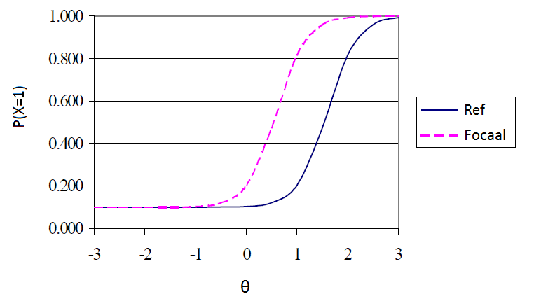
Source: Zumbo (1999), p. 20
In the case of non-uniform DIF, being 'at an advantage' or 'at a disadvantage’ varies along with a person's score for the construct that the item is measuring. For example, there is a non-uniform DIF if at a low intelligence score there is a greater chance that a candidate with a migrant background has answered an item correctly (compared to a candidate with a non-migrant background with the same score), while at a high intelligence score there is less chance of the candidate with a migrant background answering the item correctly (compared to a candidate with a non-migrant background with the same score).
An example of this is shown in Figure 6.10. If scores are below average, members from the focal group are more likely to give a correct answer than members from the reference group. If scores are above average, the reverse is true. In IRT terms, this means that both the a and b parameters differ significantly between the two groups (Steinberg, Thissen, & Wainer, 1990).
Figure 6.10. Example of an item that shows non-uniform DIF.

Source: Zumbo (1999), p. 21
Two conditions must be met before we can speak of substantial DIF. The first condition is based on significance, whereby the fit of the models is compared by means of their χ2 values. If the p value of the difference in the χ2- values of Model 3 and Model 1 (with 2 degrees of freedom) is smaller than 0.5, Model 3 is significantly better than Model 1 and there may be DIF (Swaminathan & Rogers, 1990; Zumbo, 1999).
We have already said that ‘DIF may be present': the χ2 value may become significant, for example, under the influence of the sample size, the relative size of the focal and reference groups and the difficulty of the items, (Lei et al., 2006; Swaminathan & Rogers, 1990; Zumbo, 1999). The second condition, therefore, is that there must be significant effect sizes before there can be substantial DIF (Kirk, 1996; Zumbo, 1999; Zumbo & Hubley, 1998). The difference in explained variance, ΔR2, between the different models is used for this purpose. Zumbo and Thomas (1997) give as a guideline that if ΔR2 is between 0 and .13, this indicates negligible DIF; a number between .13 and .26 indicates moderate DIF and anything >.26 indicates strong DIF. Jodoin and Gierl (2001) use the following categories: 0 - .035 is negligible, .035 - .07 is moderate and >.07 is strong. We use this latter, stricter rule of thumb in the current study. Only when both conditions (significance and a substantial effect size) are met can we speak of a substantial DIF.
The above test with 2 degrees of freedom can be seen as an omnibus test for both uniform and non-uniform DIF. One way to gain insight into the degree of uniform and non-uniform DIF is to compare the R2 values of Model 2 and Model 3. The difference in R2 values between Model 1 and Model 3 is namely additive (e.g. ΔR2M3-M1 = .10): the ΔR2 between Model 1 and Model 2 is representative of uniform DIF (e.g. ΔR2M2-M1= .08), the ΔR2 between Model 3 and Model 2 is representative of non-uniform DIF (e.g. R2M3-M2 = .02).
6.9.2. Differential Test Functioning (DTF)
With DIF, we check at item level whether the probability of a correct answer differs between two or more groups with an equal level of intelligence. However, it is also possible to see whether such differences aggregate into bias at test level: this is known as differential test functioning (DTF). Even if DIF effects are found, this does not necessarily mean that there will also be DTF: DTF may be negligible at test level if DIF does not clearly put one group at an advantage or a disadvantage. Conversely, there may be substantial DTF even if there is little evidence of DIF: small and/or insignificant effects at item level may add up to a substantial bias at test level.
This is why methods have been developed to analyse a test’s DTF. The most commonly used method is to compare the expected score at test level between groups: the expected score is then simply the sum of all odds (of a correct answer) for individual items in a test. In adaptive tests, however, this is complex. As different people are given different items and different numbers of items it is difficult to interpret and compare an expected score between groups.
The MH procedure provides a DTF statistic that is not based on expected scores but on the variance of the DIF statistics in a test or item bank. This variance, τ2, can be used to qualify the degree of DTF. Penfield and Algina (2006) use the following rule of thumb:
- τ2 < .07 indicates a small degree of DTF (approximately a maximum of 10% of the items have an absolute MH D-DIF value of 1)
- .07 < τ2 < .14 indicates an average degree of DTF
- < .14 indicates a high degree of DTF (approximately 25% or more of the items have a MH D-DIF value of 1)
To give the user even more insight into the degree of DTF, we calculated the total expected score for each person by calculating the "likelihood of a correct answer" for each person for each item shown, at the estimated θ for this person, and then adding up these likelihoods. This sum was then divided by the total number of items a person had answered: as not everyone had answered the same number of items, this ensured that everyone got a total expected score between 0 and 1. These odds were then rounded off to ensure that everyone had a score of 0 or 1. This dichotomous variable was then used as a dependent variable in logistic regression models, analogous to the DIF analyses described above. In addition, we graphically display the predicted scores based on the logistic regression model (analogous to item response functions, see Chapter 1) in order to obtain a picture of differences between groups.
6.9.3. Current study
Due to the large number of missing values inherent to the adaptive nature of the test, we conducted all analyses on the largest possible samples, i.e. on the total sample, and not on the candidate sample. Analyses of the candidate sample often yielded too few observations per item (or per item per group) to be able to detect DIF. There is more information on the background characteristics and the representativeness of the sample in section 6.8.
The DIFAS 5.0 programme (Penfield, 2005) was used for the MH procedure. For the matching criterion, the θ score per sub-test has been divided into 12 categories by cutting the θ scale into equal parts of .20 (-3 to -2.8, -2.8 to -2.6 ... et cetera, 2.8 to 3). Classifications into more categories produced too many empty cells or cells with too small numbers in the 2x2 tables in the MH procedure: other classifications were analysed but showed similar results. Zwick and colleagues (Zwick et al., 1994a; 1994b; 1995) suggested that the matching criterion should not be the estimated θ score, but the expected score across the entire item bank. This expected score can be obtained by calculating the probability of each item for the estimated θ and then summing up these probabilities across the entire item bank. All analyses from the MH procedure were also conducted using this matching criterion but as they did not produce different results, these results are not shown here.
The MH procedure appeared to mark fewer items as potential DIF items than the LR method. Therefore, when classifying the items in ETS categories, we also classified items that appeared to show significant DIF on the basis of the LR method. As the MH procedure tests for uniform DIF, we looked at the differences in χ2 values between Model 2 and Model 1 (with 1 degree of freedom).
The difR package (Magis, Beland, Tuerlinckx, & De Boeck, 2010) in R (R Core Team, 2016) was used for the logistic regression procedure. For DIF based on age we only used the LR method because only two groups can be compared in the MH procedure. With the LR method, a continuous or discrete variable (such as age) can also be used as a group variable.
There are also methods to detect DIF based on IRT, which estimate the a and b parameters for the different groups and then examine whether they differ significantly from each other (using a likelihood ratio test (LRT); Thissen, Steinberg, & Wainer, 1988; Steinberg et al., 1990). This method is less suitable in our case as making a stable estimation of the item parameters requires large samples (which is logical as the parameters are estimated per sub-group). We used the IRTLRTDIF programme (Thissen, 2001) to examine items for DIF, but the results were almost identical to those produced by the LR method. Therefore we will only show the results of the LR method. The instability of the item parameters in the IRTLRTDIF method was evidenced by several extremely large a values or very large negative or positive b values.
6.9.4. Results
6.9.4.1. Ethnicity
Table 6.49. shows the number and percentage of items that on the basis of the MH D-DIF or LR values appeared to show significant uniform DIF based on ethnicity, and the classification of items in the ETS categories.
|
Table 6.49. Results of DIF analyses on the basis of ethnicity (people with a migrant background/people with a non-migrant background). |
|||||||||||
|
ETS classification |
|||||||||||
|
MH |
LR |
Total |
C- |
B- |
A |
B |
C+ |
||||
|
Digit Sets |
Number |
10 |
13 |
14 |
2 |
4 |
197 |
7 |
1 |
||
|
% |
5 |
6 |
7 |
1 |
2 |
93 |
3 |
0 |
|||
|
Figure Sets |
Number |
7 |
5 |
8 |
0 |
6 |
179 |
1 |
1 |
||
|
% |
4 |
3 |
5 |
0 |
3 |
96 |
1 |
1 |
|||
|
Verbal Analogies |
Number |
14 |
17 |
19 |
1 |
9 |
192 |
8 |
1 |
||
|
% |
7 |
8 |
9 |
0 |
4 |
91 |
4 |
0 |
|||
|
A = small, B = moderate, C = strong |
|||||||||||
From Table 6.49 it appears that only a small number of items seem to show DIF on the basis of ethnicity, and that this applies to all three sub-tests. In addition, the right-hand panel shows that the degree of DIF is small: Digit Sets, Figure Sets and Verbal Analogies only have 3 (1%), 1 (1%) and 2 (0%) items from the C category respectively. Digit Sets, Figure Sets and Verbal Analogies have 11 (5%), 7 (4%) and 17 (8%) items from category B respectively. The least differences are found in Figure Sets: this was to be expected as this sub-test has the most culture-free type of item (see Chapters 1 and 6). It is also striking that Verbal Analogies has the most DIF items; given the verbal component of the items, more DIF effects can be expected here between people with a non-migrant background and people with a migrant background than in the other sub-tests (Schmitt & Dorans, 1990; Te Nijenhuis, 1997; Van den Berg, 2001). There are, however, the same number of B- and B+ items, which means that people with a migrant background do not seem to be clearly ‘disadvantaged’. This generally applies to all three sub-tests.
A similar picture emerged from the DTF analyses: the τ2 values for Digit Sets, Figure Sets and Verbal Analogies were .034, .014, and .055 respectively. All three values were <.07, which indicates that we may expect hardly any bias on the basis of ethnicity at item bank level.
Table 6.50. shows the results of the LR method. Once more, it is noticeable that as expected, Figure Sets had the fewest items that seemed to display DIF. There seemed to be few differences between the number of items marked as uniform DIF and non-uniform DIF. The effect sizes (two right-hand columns, Table 6.50.) showed that the items that were marked as 'potential DIF items' on the basis of their significance did not show a significant degree of DIF. Although not very relevant for small effect sizes, the R2 values showed that Digit Sets and Figure Sets mainly had non-uniform DIF items, whereas Verbal Analogies had equal numbers of items with uniform and non-uniform DIF. An inspection of the content of the potential DIF items also showed that no clear pattern could be identified in the items that appeared to show DIF.
|
Table 6.50. Results of DIF analyses on the basis of ethnicity (people with a migrant background/people with a non-migrant background) – LR method. |
|||||
|
Sig |
Average ΔR2 M3-M1 |
Max. ΔR2 |
|||
|
Digit Sets |
Number |
21 |
.0257 |
.0429 |
|
|
% |
10 |
||||
|
Figure Sets |
Number |
8 |
.0248 |
.0372 |
|
|
% |
4 |
||||
|
Verbal Analogies |
Number |
18 |
.0243 |
.0353 |
|
|
% |
8 |
||||
Figure 6.11. shows the results of the DTF analyses on the basis of logistic regression. On the basis of the figures there seems to be some difference between the expected score of candidates with a non-migrant background and candidates with a migrant background based on their θ scores. It is striking that people with a migrant background seem to be at an advantage, but when θ values are higher, persons with a non-migrant background were at a slight advantage (non-uniform DTF). Formal χ2 tests only showed any indication of DIF at test level in Figure Sets (χ2(2) = 10.9, p = .00) and Verbal Analogies (χ2(2) = 20.4, p = .00) (In Digit Sets, χ2(2) = 6.0, p = .05). However, it seems that we found significant effects because of the larger sample: ΔR2 were .0013, .0028 and .0000 for Digit Sets, Figure Sets and Verbal Analogies respectively. At test level, there seems to be little or no bias on the basis of ethnicity.
In view of the fact that persons with a migrant background do not appear to be clearly disadvantaged, that few or no items seemed to show substantial DIF and that these small differences at test or item bank level hardly lead to differences, we have decided not to remove items from the item banks on the basis of the DIF analyses.
Figure 6.11. Expected scores on the basis of DTF analyses - ethnicity.
Digit Sets Figure Sets


Verbal Analogies
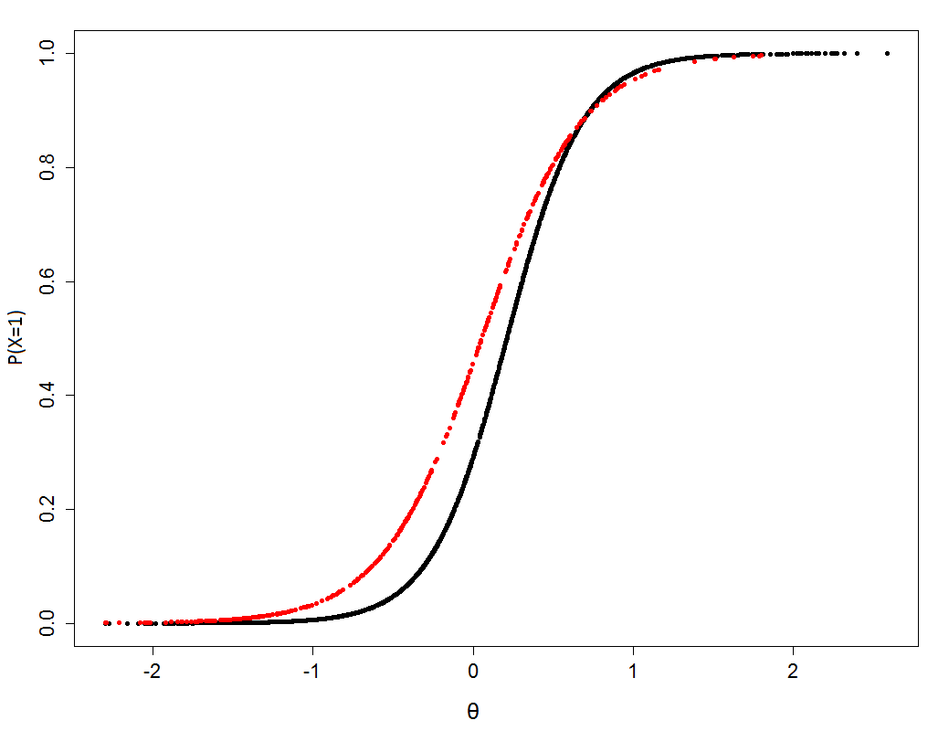
Non-migrant Migrant
6.9.4.2. Gender
Table 6.51. shows the number and percentage of items that on the basis of the MH D-DIF or LR values appeared to show significant uniform DIF based on ethnicity, and the classification of items in the ETS categories.
|
Table 6.51. Results of DIF analyses on the basis of gender (men/women). |
|||||||||||
|
ETS classification |
|||||||||||
|
MH |
LR |
Total |
C- |
B- |
A |
B |
C+ |
||||
|
Digit Sets |
Number |
15 |
20 |
18 |
2 |
9 |
193 |
6 |
1 |
||
|
% |
7 |
9 |
8 |
1 |
4 |
91 |
3 |
0 |
|||
|
Figure Sets |
Number |
11 |
10 |
13 |
0 |
7 |
174 |
6 |
0 |
||
|
% |
6 |
5 |
7 |
0 |
4 |
93 |
3 |
0 |
|||
|
Verbal Analogies |
Number |
13 |
22 |
22 |
0 |
8 |
191 |
14 |
0 |
||
|
% |
6 |
10 |
11 |
0 |
4 |
90 |
7 |
0 |
|||
|
A = small, B = moderate, C = strong |
|||||||||||
Table 6.51. shows that in each of the three sub-tests approximately 10% of the items show gender-based DIF. However, the right-hand panel shows that the degree of DIF is small: only Digit Sets has items from the C category, but this is only 3 (1%). Digit Sets, Figure Sets and Verbal Analogies have 15 (7%), 13 (7%) and 22 (11%) items from category B respectively. Furthermore, we see that men and women are not clearly at an advantage or a disadvantage as there are approximately the same number of items in the - and + categories. A similar picture emerged from the DTF analyses: the τ2 values for Digit Sets, Figure Sets and Verbal Analogies were .039, .016, and .021 respectively. There were no distortions on the basis of gender at item bank or test level.
We can draw the same conclusions on the basis of the LR method (Table 6.52.). Approximately 10% of the items in each sub-test shows (uniform/non-uniform) DIF. Verbal Analogies mainly seems to show uniform DIF. The effect sizes also showed that DIF was generally negligible with regard to gender. A review of the R2 values of the different models showed that uniform and non-uniform DIF was found in equal measure in Digit Sets and Figure Sets, whereas there was mainly uniform DIF in Verbal Analogies (with women being the main beneficiaries).
Both Digit Sets and Verbal Analogies had 1 item that displayed substantial DIF (ΔR2M3-M2 > .07, see right-hand column). This appeared to involve items that had not yet been shown to candidates, but had only been seen by people in the calibration study. The item in Digit Sets had already been removed from the item bank on the basis of other item fit statistics during the recalibration in July 2016. To collect more data in actual selection situations we decided to keep the Verbal Analogies item in the item bank.
|
Table 6.52. Results of DIF analyses on the basis of gender (men/women) – LR method. |
|||||
|
Sig |
Average ΔR2 M3-M1 |
Max. ΔR2 |
|||
|
Digit Sets |
Number |
22 |
.0270 |
.1182 |
|
|
% |
10 |
||||
|
Figure Sets |
Number |
15 |
.0181 |
.0417 |
|
|
% |
8 |
||||
|
Verbal Analogies |
Number |
20 |
.0256 |
.1135 |
|
|
% |
9 |
||||
Figure 6.12. shows the results of the logistic DTF analyses for gender.
Figure 6.12. Expected scores on the basis of DTF analyses – gender.
Digit Sets Figure Sets


Verbal Analogies

Man
Female
Based on a visual inspection of the predicted probabilities for men and women, the distance between the two lines seems to indicate uniform DTF: women are at a disadvantage compared to men, and the bias seems to be greatest in the case of the Figure Sets. Although the χ2 tests initially seemed to indicate DTF, the R2 values once more indicated extremely small effects (.0000, .0140, .0000). Here also, there seems little or no bias on the basis of gender at test level.
Due to the above results, we did not remove any items from the item bank on the basis of the DIF analyses for gender.
6.9.4.3. Age
Table 6.53. shows the results of the DIF analyses on the basis of age. More items were marked as potential DIF items than in the ethnicity and gender analyses. However, the average effect sizes can be qualified as small according to the classification of Jodoin and Gierl (2001). In total there were 5 items (2%) with an average degree of DIF in Verbal Analogies, 8 items (4%) in Digit Sets and 2 items (1%) in Figure Sets.
|
Table 6.53. Results of DIF analyses on the basis of age – LR method. |
|||||
|
Sig |
Average ΔR2 M3-M1 |
Max. ΔR2 |
|||
|
Digit Sets |
Number |
39 |
.0245 |
.0673 |
|
|
% |
18 |
||||
|
Figure Sets |
Number |
20 |
.0188 |
.0381 |
|
|
% |
11 |
||||
|
Verbal Analogies |
Number |
36 |
.0235 |
.0585 |
|
|
% |
17 |
||||
Inspection of the R2 values showed that Digit Sets had slightly more items that mainly showed uniform DIF than non-uniform DIF. When there were non-uniform DIF items, older people were mainly at a disadvantage. In the case of non-uniform items, there was no clear advantage for either older or young people.
In Figure Sets, more items showed uniform DIF than non-uniform DIF, whereby older people were disadvantaged approximately as often as younger people. The majority of the items that showed non-uniform DIF favoured older people with high abstract intelligence and young people with low abstract intelligence.
Most items in Verbal Analogies showed uniform DIF, whereby older people were disadvantaged approximately as often as younger people in these uniform DIF items. As with Figure Sets, there was no clear advantage for either older or young people in the case of non-uniform items.
Figure 6.13. shows the results of the logistic DTF analyses for age: the predicted values are presented for the age groups 'up to 25', '25 to 45' and '>45’ purely for visual purposes and age is included in the analyses as a continuous variable.
Figure 6.11. shows that there seem to be hardly any differences in the scores expected on the basis of age. This was also shown by the logistic regression (χ2(2) = 3.8, p = .15). In Figure Sets, it seems to be mainly older people with a lower abstract intelligence level who are disadvantaged in comparison with the youngest category. The difference disappears at the higher levels. The middle age category seems to be generally advantaged in comparison with the other two groups. Although there seemed to be DTF on the basis of the significance level (χ2(2) = 19.4, p = .00), the effect size was negligible (ΔR2M3-M1 = .0035). In the case of Verbal Analogies, the figure shows that the middle and youngest categories appear to differ little in terms of expected scores, while the older people appear to be disadvantaged across the entire θ scale. However, the differences turned out to be negligible (χ2(2) = 24.5, p = .00, ΔR2M3-M1 = .0000). On the basis of these analyses, it seems that we may expect little age-based bias at test level.
Figure 6.13. Expected scores on the basis of DTF analyses – age.
Digit Sets Figure Sets


Verbal Analogies

< 25 years
25 to 45 years
> 45 years
6.9.5. Conclusions on DIF in ACT General Intelligence
On the basis of various methods - using relatively strict criteria - this study has shown that we cannot expect to find any substantial DIF in ACT General Intelligence on the basis of ethnicity, gender and age. There were indications of potential DIF for a number of items, but the effect sizes indicated only slight differences between groups. Furthermore, groups did not appear to be consequently put at either an advantage or a disadvantage. DTF analyses at test and item bank level showed that we can expect little bias at test level on the basis of ethnicity, age and gender.
6.10 Research into person fit
6.10.1. Introduction
In the sections on item fit, we checked whether the items and their estimated parameters behave according to the established IRT model. We can examine person fit in a similar manner: person fit is about whether people’s answer patterns are consistent with the IRT model. A candidate’s answer patterns can be predicted on the basis of an IRT model. Unlikely or inconsistent answer patterns can be identified using person-fit statistics. For example, an answer pattern would be inconsistent if someone has answered all the easier questions incorrectly and the more difficult questions correctly. Person fit is important for the validity of the obtained test scores: θ is determined on the basis of the test participant's answer pattern, (section 1.4.2.), and since important decisions depend on this estimate of θ (e.g. whether or not the candidate gets the job), it is important to be sure that the answer pattern has been established in the 'correct' manner. Person fit is a direct reflection of the validity of test scores obtained at individual level. In other words, if person-fit statistics reveal a deviating answer pattern, this raises doubts concerning the correctness of the test results.
6.10.2. Person fit in adaptive tests
The literature speaks of different measures that can detect deviating score patterns, each with their own pros and cons. We have therefore chosen to use two measures: the CUSUM procedure and the number of Guttman errors.
6.10.2.1. CUSUM
In an adaptive test, people can obtain the same estimated θ in different ways, based on different answer patterns. There are various causes for this, such as carelessness or guessing. For example: one person may first answer a number of questions incorrectly (due to carelessness) and then answer some correctly, while another person may, for example (more in conformity with the model) have one right, then one wrong et cetera, and still end up with the same θ. One person fit measurement method that gives us good insight into this is the “cumulative sum” procedure (CUSUM; Van Krimpen-Stoop & Meijer, 2002). Although there are many person-fit statistics in the literature, we choose the CUSUM method to examine person fit in ACT General Intelligence.
The CUSUM procedure works as follows: Based on the estimated θ after completing the ACT General Intelligence, it is possible to calculate the probability of a correct answer (P) for each item: this is the expected score (E). The residual (O - E) can be calculated for each observed score (O). The statistical T can be calculated on this basis: this is simply the residual divided by the total number of items answered.
This T score and the residuals are then used to create two series, one with positive residuals and one with negative residuals. The series of positive residuals has a minimum of 0, the series of negative residuals has a maximum of 0 (see Figure 6.14. and 6.15.).
Figure 6.14. Formulas of the CUSUM procedure.

Source: Egberink (2010, p. 56)
Figure 6.15. Example of the CUSUM procedure.
Source: Egberink (2010, p. 57)
This person has answered 20 items, whereby the first item was answered incorrectly (O = 0), while the expected score (E = ) was .411. Therefore, for the first item, T is (0 - .411) / 20 = -.021. This residual is subtracted from the C- series, not from the C+ series as this series has a minimum of 0. The same principle is repeated in this way for every item. This example clearly shows that C- only becomes a large negative number if the score is consistently lower than predicted, and C+ only becomes a large positive number if the score is higher than predicted. A person who is careless when taking the test will have relatively lower C-values while someone who has managed to get hold of the answers to a test will have relatively higher C+ values. The CUSUM procedure therefore accurately charts whether people are scoring ‘too high’ or ‘too low’ on an item.
We have calculated the above series for everyone who has taken ACT. However, it is still necessary to determine test limits for C- and C+ stipulating when an answer pattern can be considered as “deviating”. We used one of the methods of Van Krimpen-Stoop and Meijer (2002) that is commonly used in the literature. We simulated a thousand item responses according to the 2PL model (the IRT model used in ACT): this enabled us to determine the values of C- and C+ that can be expected from answer patterns according to the IRT model. Subsequently, a bootstrap procedure (with 1000 retractions with reversal) was carried out to approximate the sample distributions of the 5th percentile (C-) and the 95th percentile (C+) (the bootstrap distributions). The medians of these distributions then determined the test limits.
Eventually, this meant that an answer patterns was considered as being deviating when C+ exceeded .2286 in Digit Sets, .2618 in Figure Sets and 2366 in Verbal Analogies. For C- an answer pattern was deviating if it was lower than -.2339 in Digit Sets, -.2616 in Figure Sets and -.2429 in Verbal Analogies.
6.10.2.2. Number of Guttman errors
The second method we chose was the number of Guttman errors (1950). The advantage of this measurement tool is that it is simple, intuitive, and has been shown to work well for detecting inconsistent answer patterns (Meijer, 1994). According to IRT, a person who answers an item with a difficulty degree (b) of -1 correctly, must also answer an item with a difficulty degree -1.5 correctly. A Guttman error is an answer that does not correspond with the IRT model. It is easiest to illustrate this with an example. An imaginary person has answered 5 items with b values (ranked from difficult to easy) of 2, 1, 0.5, 0, -0.1 with the following answer pattern: 11010. This person has made one Guttman error: he or she answered the fourth – relatively more difficult – item (b = 0) correctly and the third – relatively easier – item (b = 0.5) incorrectly. The answer pattern therefore does not correspond to the model. The number of Guttman errors depends on the length of a person’s answer pattern (Meijer, 1994). Because in ACT General Intelligence, different people may be set a different number of items, we have used the standardised measure, which corrects for this. This measure ranges from 0 to 1, whereby 0 means ‘no person misfit’ and 1 is a score pattern that deviates entirely from what one could expect on the basis of the IRT model.
This measure is a non-parametric statistic and therefore has no theoretical sample distribution. In order to be able to determine a critical value at which we consider the number of Guttman errors as being 'too high' (and therefore the answer pattern as 'deviating'), the same bootstrap procedure was used as for the test boundaries of the CUSUM procedure. In Digit Sets a value ≥ .8184 can be considered as deviating; this value is ≥ .7890 in Figure Sets and ≥ .8764 in Verbal Analogies.
6.10.3. Expectations
The test limits described above were used to determine the percentage of the sample that showed a deviating answer pattern. A second application of person fit statistics is to distinguish between groups that show deviant response behaviour: if certain groups (e.g. men versus women) systematically show more deviant answer patterns, their scores will be less valid than those of the other groups. Therefore we have also compared the person fit values of different groups to each other.
For the validity of the response patterns ̶ and therefore the estimates of θ ̶ there should be no differences in the C- and C+ values based on gender and ethnicity (people with a migrant background/people with a non-migrant background).
This is slightly different in the case of the education levels variable: it is to be expected that people with a higher level of education will have a higher level of intelligence than people with a lower level of education. One feature of ACT is that the probability of answering an item correctly is basically about 50%. As ACT starts at a difficulty of -0.5, the probabilities for higher educated people (with higher θs) will be much higher at the beginning. People with a higher level of education (higher θ) will therefore first answer a number of items correctly and will therefore have no negative residuals, so that C-will remain at 0 for longer at the beginning of the tests. This will result in them having a lower C- than people with a lower level of education. It is less easy to predict C+. After a number of items, the likelihood that a person with a higher level of education will answer an item correctly will be approximately 50%, leading to both positive and negative residuals. People with a lower education level are also more likely to be asked questions that give them a 50% chance of answering correctly. This makes it unclear whether their C+ will be higher or lower than that of people with a higher education level.
With regard to the number of Guttman errors, it would back up the validity of ACT General Intelligence if no differences were found with respect to gender, ethnicity and education level.
As the item parameters were calibrated for the entire sample (consisting of persons from the calibration sample and 'real' candidates from Ixly’s system), the analyses were conducted for the total sample and the candidate sample.
6.10.4. Results
Both the total sample (calibration and candidate sample) and the candidate sample were analysed. There is more information on background characteristics in section 6.8.
6.10.4.1. CUSUM: number of deviating answer patterns and differences between groups
Because we used the 95th percentile, a percentage of 5% 'deviating' answer patterns is acceptable. However, percentages under/above the critical values of C- and C+ respectively were generally smaller (Table 6.54.).
|
Table 6.54. Percentage deviating answer patterns based on the CUSUM procedure. |
||
|
Total samplea |
Candidate sampleb |
|
|
Digit Sets |
3.4 |
1.3 |
|
Figure Sets |
5.3 |
2.3 |
|
Verbal Analogies |
3.6 |
3.8 |
|
a N = 5079-5238. b N = 2532-2534. |
||
Table 6.55 shows the percentages of deviating answer patterns for different groups. It is striking that the percentages are considerably higher in the total sample than in the data obtained from 'real' users of the test. The total sample consisted partly of people who had participated in research for a remuneration (i.e. the people from the calibration sample): it is therefore quite possible that they took the test less seriously, which can be seen in the higher percentages of deviating score patterns.
We conducted χ2 tests to examine whether the proportions of deviating score patterns varied on the basis of ethnicity, gender and education level. No significant differences were found between people with a migrant background and people with a non-migrant background or between men and women in the candidate sample (Table 6.55.) There were differences, however, between men and women in the total sample (Figure Sets) and between different levels of education (Figure Sets and Verbal Analogies).
|
Table 6.55. Percentage of deviating answer patters based on the CUSUM procedure according to ethnicity, gender and education level. |
||||||||||||
|
Ethnicity |
Gender |
Education level |
||||||||||
|
Calibration sample |
Total |
Candidate |
Candidate |
|||||||||
|
Non-migrant backgrounda |
Migrant backgrounda |
Manb |
Womanb |
Manc |
Womanc |
Level 2d |
Level 3d |
Level 6d |
Level 7d |
|||
|
Digit Sets |
5.4 |
5.1 |
3.2 |
3.9 |
1.4 |
1.1 |
1.5 |
1.4 |
1.0 |
.3 |
||
|
Figure Sets |
8.2 |
10.5 |
4.8* |
6.5* |
2.2 |
2.4 |
3.9 |
3.0** |
.8** |
.6** |
||
|
Verbal Analogies |
3.2 |
4.2 |
3.9 |
3.5 |
4.1 |
4.2 |
6.9** |
4.8** |
2.7 |
1.2** |
||
|
** p < .01 (two-tailed). bNmen = 2507-2587, Nwomen = 2212-2307. cNmen = 1456-1457, Nwomen = 746-748. d NLevel 2 = 203, NLevel 3 = 1093-1094, NLevel 6 = 399-401, NLevel 7 = 326-327. |
||||||||||||
In order to get an idea of the size of the differences, we took Cohen's d as a measure of effect size for the difference between men and women, and η2 for educational level. In the Figure Sets sub-test, the difference between men and women in the total sample was small (d = -.07). The difference on the basis van education level was extremely small for both Figure Sets and Verbal Analogies (η2 = .007). In Figure Sets, the only significant difference was between the education level 3: upper secondary education and education level 6: bachelor or equivalent groups; in Verbal Analogies, the percentage of deviating patterns deviated significantly from the percentage in the education level 2: lower secondary education and education level 3: upper secondary education groups.
On the basis of these results, we can conclude that relatively few deviating answer patterns can be observed in ACT General Intelligence. Little or no differences were found between groups. Only the education level 2: lower secondary education group showed more deviating score patterns than we would expect on the basis of chance. This means that the answer patterns/scores for ACT General Intelligence can be considered valid.
6.10.4.2. CUSUM: differences between groups in C- and C+
We did not find any significant differences in C-values between people with a migrant background and people with a non-migrant background. This means that people with a migrant background did not answer questions incorrectly any more often than people with a non-migrant background than we could expect on the basis of the model. We did find small, marginally significant differences in C+ values between people with a migrant background and people with a non-migrant background In Figure Sets (d = -.11, p = .09) and Verbal Analogies (d = -.12, p = .05). From the minus and plus signs of the effect sizes d, we can conclude that people with a migrant background are 'at a disadvantage' in the Figure Sets and 'at an advantage' in Verbal Analogies. We can generally conclude that there are no differences with respect to ethnicity in the consistency of answer patterns (and therefore the θ estimates).
|
Table 6.56. differences in C- and C+ according to ethnicity. |
|||||||||||
|
C- |
C+ |
||||||||||
|
Non-migrant background |
Migrant background |
d |
Non-migrant background |
Migrant background |
d |
||||||
|
M |
SD |
M |
SD |
M |
SD |
M |
SD |
||||
|
Digit Sets |
-.16 |
.05 |
-.16 |
.05 |
.08 |
.16 |
.05 |
.15 |
.05 |
.06 |
|
|
Figure Sets |
-.18 |
.05 |
-.18 |
.04 |
.05 |
.17 |
.06 |
.18 |
.06 |
-.11† |
|
|
Verbal Analogies |
-.14 |
.05 |
-.14 |
.05 |
-.02 |
.13 |
.05 |
.13 |
.07 |
.12* |
|
|
*p <.05 (two-tailed), ** p < .01 (two-tailed). aNnon-migrant background = 2222-2355, Nmigrant background = 296-331 (calibration sample). |
|||||||||||
We only found significant C- differences between men and women in Figure Sets and Verbal Analogies, in both the total sample and the candidate sample. The differences were small according to Cohen’s (1988) guidelines. Men had higher C-values for Figure Sets and lower C-values for Verbal Analogies. We only found a small significant difference in C+-values for Figure Sets in the total sample. In general, we can therefore conclude that men and women’s answer patterns were equally consistent.
|
Table 6.57. Differences in C- and C+ according to gender. |
|||||||||||
|
Totala |
Candidatesb |
||||||||||
|
Men |
Women |
d |
Men |
Women |
d |
||||||
|
C- |
M |
SD |
M |
SD |
M |
SD |
M |
SD |
|||
|
Digit Sets |
-.16 |
.05 |
-.16 |
.05 |
.05 |
-.16 |
.05 |
-.16 |
.05 |
.01 |
|
|
Figure Sets |
-.17 |
.05 |
-.17 |
.05 |
.06* |
-.17 |
.05 |
-.17 |
.05 |
.09* |
|
|
Verbal Analogies |
-.14 |
.05 |
-.14 |
.05 |
-.08** |
-.15 |
.06 |
-.14 |
.06 |
-.11* |
|
|
C+ |
|||||||||||
|
Digit Sets |
.15 |
.04 |
.15 |
.04 |
-.02 |
.15 |
.03 |
.15 |
.03 |
.07 |
|
|
Figure Sets |
.17 |
.05 |
.17 |
.06 |
-.06* |
.16 |
.04 |
.16 |
.04 |
.05 |
|
|
Verbal Analogies |
.14 |
.05 |
.14 |
.05 |
.00 |
.15 |
.04 |
.15 |
.04 |
.03 |
|
|
*p < .05 (two-tailed), **p < .01 (two-tailed). bNmen = 1456-1457, Nwomen = 746-748. |
|||||||||||
Table 6.58. shows the differences in C- and C+ between the different education levels. As predicted, C-values decreased in higher education levels in all three sub-tests. The differences are large (η2, last column). There is also a negative relation between education level and the height of C+ values, for Figure Sets and Verbal Analogies: the WO group has significantly lower values than the education level 2 and education level 3 groups. The differences are smaller than for the C-values, based on the effect sizes.
As described above, these differences cannot be attributed to a lack of validity, but are the result of ACT’s adaptive procedure in combination with the fact that education level is related to intelligence.
|
Table 6.58. Differences in C- and C+ according to education level. |
|||||||||
|
Level 2a |
Level 3a |
Level 6a |
Level 7a |
η2 |
|||||
|
M |
SD |
M |
SD |
M |
SD |
M |
SD |
||
|
C- |
|||||||||
|
Digit Sets |
-.18b |
.04 |
-.17c |
.04 |
-.15b,c,d |
.05 |
-.13b,c,d |
.05 |
.122** |
|
Figure Sets |
-.19b |
.04 |
-.18c |
.04 |
-.16b,c,d |
.05 |
-.13b,c,d |
.05 |
.147** |
|
Verbal Analogies |
-.17b |
.04 |
-.17c |
.05 |
-.12b,c |
.06 |
-.10b,c |
.05 |
.217** |
|
C+ |
|||||||||
|
Digit Sets |
.15b |
.03 |
.15c |
.03 |
.15b,c |
.04 |
.15 |
.04 |
.006** |
|
Figure Sets |
.16b |
.03 |
.16c |
.04 |
.16 |
.04 |
.15b,c |
.04 |
.014** |
|
Verbal Analogies |
.16b |
.04 |
.16c |
.04 |
.14b,c |
.04 |
.13b,c |
.04 |
.064** |
|
** p < .01 (two-tailed). d NLevel 2 = 203, NLevel 3 = 1093-1094, NLevel 6 = 399-401, NLevel 7 = 326-327. |
|||||||||
6.10.4.3. Number of Guttman errors: number of deviating answer patterns and differences between groups
Analogous to the analyses for the C- and C+ values, we first looked at 'too high' values for the number of Guttman errors: because we used the 95th percentile, a percentage of 5% 'deviating' answer patterns is acceptable. As Table 6.59. shows, however, these percentages are very small. The answer patterns scarcely deviate on the basis of the number of Guttman errors.
|
Table 6.59. Percentage deviating answer patterns on the basis of the number of Guttman errors. |
||
|
Total samplea |
Candidate sampleb |
|
|
Digit Sets |
0.32 |
0.04 |
|
Figure Sets |
1.05 |
0.20 |
|
Verbal Analogies |
0.38 |
0.28 |
|
a N = 5039-5270. b N = 2526-2556. |
||
We also looked at the differences between groups in terms of the number of Guttman errors: these are shown in Table 6.60.
|
Table 6.60. Percentage of deviating answer patterns based on the number of Guttman errors according to ethnicity, gender and education level. |
||||||||||||
|
Ethnicity |
Gender |
Education level |
||||||||||
|
Calibration sample |
Total |
Candidate |
Candidate |
|||||||||
|
Non-migrant backgrounda |
Migrant backgrounda |
Manb |
Womanb |
Manc |
Womanc |
VMBOd |
MBOd |
HBOd |
WOd |
|||
|
Digit Sets |
0.51 |
1.20 |
0.27 |
0.43 |
0.00 |
0.13 |
0.00 |
0.00 |
0.25 |
0.00 |
||
|
Figure Sets |
1.77 |
2.73 |
1.09 |
1.13 |
0.34 |
0.00 |
0.99 |
0.09 |
0.00 |
0.31 |
||
|
Verbal Analogies |
0.43 |
1.03 |
0.37 |
0.37 |
0.21 |
0.27 |
0.00 |
0.09 |
0.50 |
0.31 |
||
|
aNnon-migrant background = 2202-2366, Nmigrant background = 293-332. bNmen = 2480-2596, Nwomen = 2212-2319. cNmen = 1453-1463, Nwomen = 746-754. d NLevel 2 = 203-205, NLevel 3 = 1093-1097, NLevel 6 = 398-406, NLevel 7 = 324-329. |
||||||||||||
In the χ2 tests, we found no significant differences in terms of ethnicity, gender and education levels: however, because the numbers identified as 'deviant' were so low, we must avoid drawing overly confident conclusions from them.
6.10.4.4. Number of Guttman errors: differences between groups
Significant differences were found between people with a migrant background and people with a non-migrant background in the Digit Sets and Figure Sets sub-tests; people with a migrant background generally showed slightly more deviant score patterns than people with a non-migrant background, although the effect sizes indicated that the effects are small.
|
Table 6.61. Differences in the number of Guttman errors according to ethnicity. |
|||||
|
Non-migrant background |
Migrant background |
d |
|||
|
M |
SD |
M |
SD |
||
|
Digit Sets |
.26 |
.16 |
.29 |
.18 |
-.22** |
|
Figure Sets |
.33 |
.18 |
.35 |
.18 |
-.13* |
|
Verbal Analogies |
.23 |
.15 |
.24 |
.16 |
-.06 |
|
*p <.05 (two-tailed), ** p < .01 (two-tailed). aNnon-migrant background = 2115-2311, Nmigrant background = 292-323. |
|||||
In the total sample (both the calibration sample and 'real' candidates from Ixly’s system), small significant differences were found for all three sub-tests, whereby women generally showed slightly more deviant score patterns than men. No differences between men and women were found in the sample that consisted only of persons who had taken the adaptive test in real selection situations (Table 6.62.).
|
Table 6.62. Differences in the number of Guttman errors according to gender. |
|||||||||||
|
Totala |
Candidatesb |
||||||||||
|
Men |
Women |
d |
Men |
Women |
d |
||||||
|
M |
SD |
M |
SD |
M |
SD |
M |
SD |
||||
|
Digit Sets |
.21 |
.16 |
.22 |
.16 |
-.09** |
.16 |
.14 |
.16 |
.14 |
.05 |
|
|
Figure Sets |
.25 |
.18 |
.28 |
.18 |
-.14** |
.19 |
.16 |
.18 |
.15 |
.06 |
|
|
Verbal Analogies |
.20 |
.17 |
.21 |
.16 |
-.08** |
.18 |
.17 |
.19 |
.18 |
-.05 |
|
|
** p < .01 (two-tailed). a nmen = 2462-2550 Nwomen = 2145-2778. bNmen = 1448-1454, Nwomen = 746. |
|||||||||||
When looking at education level, we only found significant differences in the number of Guttman errors in Verbal Analogies. The education level 2: lower secondary education and education level 3: upper secondary education groups had more deviating answer patterns than the education level 6: bachelor or equivalent and education level 7: master or equivalent groups, but the effect size indicated that this effect was small (Table 6.63).
|
Table 6.63. Differences in the number of Guttman errors according to education level. |
|||||||||
|
Level 2a |
Level 3a |
Level 6a |
Level 7a |
η2 |
|||||
|
M |
SD |
M |
SD |
M |
SD |
M |
SD |
||
|
Digit Sets |
.15 |
.13 |
.16 |
.13 |
.16 |
.15 |
.16 |
.15 |
.001 |
|
Figure Sets |
.19 |
.17 |
.19 |
.15 |
.17 |
.15 |
.20 |
.17 |
.001 |
|
Verbal Analogies |
.20c |
.16 |
.20d |
.16 |
.15c,d |
.18 |
.14c,d |
.19 |
.019** |
|
** p < .01 (two-tailed). d NLevel 2 = 202-203, NLevel 3 = 1092-1094, NLevel 6 = 398-401, NLevel 7 = 320-326. |
|||||||||
The findings for the number of Guttman errors are in contrast to the findings for the CUSUM procedure with respect to education level: however, as already indicated, this can be explained by the specific characteristics of the CUSUM procedure which lead us to expect differences between educational levels.
6.10.5. Conclusions on person fit
This study has shown that after applying these two measures (C- and C+ from the CUSUM method and the number of Guttman errors) we see few deviating answer patterns in ACT General Intelligence. People therefore displayed answer patterns that were consistent with the chosen IRT model. As a person’s score is determined on the basis of their answer pattern, these findings support the validity of test scores obtained at individual level.
We also found little or no differences between different groups with regard to background characteristics (ethnicity, gender and education level). This means that the scores for these different groups can be considered equally valid. This study therefore contributes to the validity of test scores obtained in ACT General Intelligence.
6.11 General conclusions regarding construct validity
The results described in this chapter and section 1.5.1. provide clear proof of the construct validity of ACT General Intelligence. First of all, the good degree of item fit and the fit of the chosen IRT model are an indication of the validity of the model used. By means of the intercorrelations between the sub-tests, we have demonstrated convergent validity and unidimensionality. This was also shown by a study where a single factor model was compared with a two-factor model. In addition, the structure of the three sub-tests was upheld in different groups. We found further evidence of the assumed g factor in ACT General Intelligence in a range of studies. We have also demonstrated the divergent validity of the ACT General Intelligence through relations with personality. Convergent validity was also demonstrated in this study (with the Openness factor), as well as in two studies on the relations with reading comprehension and reaction times.
Congruent validity was demonstrated in a study with the MCT-H (Bleichrodt & Van den Berg, 1997, 2004): the correlations between the ACT General Intelligence sub-tests and the MCT-H sub-tests were high (average .60, corrected for (un)reliability average .74). The g scores could hardly be distinguished from each other: the correlations between the g score based on ACT General Intelligence and the g score based on MCT-H was .80 (.95 after correction for (un)reliability). Structural models also showed that the structure of the two tests was very similar, as was the high overlap between the two g-scores (r = .99).
Differences in intelligence that can be expected on the basis of education level can also be found in ACT General Intelligence. These findings show that ACT General Intelligence scores seem to correspond to actual differences between groups and that the intended construct – intelligence – including these actual differences between groups is what is actually being measured. This also applies to age-based differences, where predictions about the relation between age and intelligence were largely confirmed by ACT General Intelligence; this conclusion also applies to differences that we found on the basis of gender. However, the differences found in relation to age and gender were small to medium in all cases: this means that ACT General Intelligence can be used for all age groups and for both men and women.
The fact that people with a non-migrant background and people with a migrant background did not seem to differ in terms of their θs in the Figure Sets sub-test provides further confirmation that Figure Sets is the most culture-free of the three sub-tests, as we had predicted on the basis of the literature. The differences on the basis of ethnicity were small to average and this may be taken into account when interpreting scores (see also Chapter 4 on this subject).
Research into differential item functioning and differential test functioning (DTF) showed that few distortions in item responses on the basis of age, gender and ethnicity are to be expected when using ACT General Intelligence. This is an important finding with regard to the fairness of this test. This study has shown that ACT General Intelligence is suitable for use among different groups. The same conclusion can be drawn when we examine person fit: only a few people had score patterns that deviated from the theoretically assumed model. There were also few differences in the number of deviating score patterns based on gender, level of education and ethnicity.
7. Criterion Validity
Criterion or predictive validity refers to the predictive value of test scores (Cotan, 2009). In order to determine the criterion validity, studies were conducted to examine the relationship between ACT General Intelligence and a range of constructs from various domains. These will be discussed below.
In this chapter, we will first discuss a study of the relationships between scores for ACT General Intelligence and a number of outcome measures for which it has been repeatedly demonstrated that they can be predicted by intelligence. Some of these outcome measures – namely those related to work – are particularly important with regard to the objective of the ACT General Intelligence test (i.e. selection purposes) and the professional area for which the test was developed (HRM, selection and assessment).
Section 7.2. describes a study of the relationship between intelligence and academic performance. In view of the aforementioned test objective and the professional area for which ACT was developed, these results may seem less relevant. Academic performance, however, appears to be strongly related to work performance. In academic research, therefore, academic performance is often considered as equivalent to work performance, but mostly with regard to students/universities (Kuncel, Hezlett, & Ones, 2004). For example, university citizenship behavior (Gehring, 2006; Zettler, 2011) and counterproductive academic behavior (Marcus, Lee, & Ashton, 2007; Zettler, 2011) are the counterparts of organizational citizenship behavior (Chiaburu, Oh, Berry, Li, & Gardner; Katz, 1964; Organ, 1988) and counterproductive work behavior (Rotundo & Spector, 2010). This is because factors (e.g. motivation, personality, intelligence) that are assumed to influence academic performance also seem to influence work performance (Kuncel et al., 2004). In this way, this research can contribute to the criterion validity of ACT General Intelligence.
Although these studies were not conducted under the same conditions as those for which the test was intended (i.e. selection situations), the data can still contribute to the criterion validity of ACT General Intelligence. Firstly, it is not uncommon to use students or populations other than the target populations in the development and validation of psychological tests (e.g. the FFPI: Hendriks, 1997; Hendriks, Hofstee, De Raad, & Angleiter, 1999). In addition, a test supervisor was present during the first study, which partly simulated the experience of taking the test in a test room, this environment being likely to make the candidates take the test seriously.
A final remark relates to the study sample described in section 7.1. This sample is the same as the sample used to examine convergent validity (section 6.5.1.). As this concerns different types of validity, we have chosen to describe the studies in different chapters. The research procedure and sample characteristics are described in section 6.5.1.2.
7.1. Research into health, socio-economic status, work and school achievement
‘General Intelligence' is an extremely broad competence that gives people the ability to solve problems, make connections between things, think abstractly, understand complex ideas and learn quickly, also from previous experiences (Gottfredson, 1997, p. 13). This makes it a very general functional competence that enables people to achieve generally appreciated goals (Gottfredson, 1997). We can therefore expect it to affect a wide range of life areas, including general health (Gottfredson, 2004), attaining higher socio-economic status (Strenze, 2007), work characteristics (e.g. work complexity; Gottfredson, 1997) and job performance (Schmidt & Hunter, 2004). The relationships between ACT General Intelligence scores and the aforementioned outcomes have been investigated to provide evidence of the criterion validity of ACT General Intelligence.
7.1.1. Hypotheses
Health
A link has been established between intelligence and health, particularly in terms of lifestyle, risk of disease and life expectancy (Gottfredson, 2004; Gottfredson & Deary, 2004). For example, a weak negative relationship is generally found between intelligence and unhealthy lifestyles such as smoking (Gottfredson & Deary, 2004). Based on this, we expected to find a weak relationship between intelligence and smoking behaviour.
Socio-economic status
A person’s socio-economic status says something about his or her place in society; their place on the 'social ladder'. Important indicators of this include level of education, occupation and income.
The relationship between intelligence and level of education is evident and has been demonstrated many times (see for example Ceci, 1991; Herrnstein & Murray, 1994; Neisser et al., 1996, Sewell & Shah, 1967). Based on Strenze’s (2007) meta-analysis, we may expect intelligence to have a strong effect on level of education (approximately r = .46).
Many studies have shown a direct positive relationship between intelligence and income (e.g. Ceci & Williams, 1997; Heckman, Stixrud, & Urzua, 2006; Herrnstein & Murray, 1994; Scullin, Peters, Williams, & Ceci, 2000). Reasonably recent meta-analyses have shown that the correlation between income and intelligence will be around .21 (Strenze, 2007) and .27 (Ng et al., 2005). We can therefore expect a comparable correlation between income and ACT General Intelligence scores.
The relationship between intelligence and professional status is also clearly described in the literature (for overview articles, see Judge, Higgins, Thoresen, and Barrick, 1999 and Schmidt and Hunter, 2004). According to Strenze’s (2007) meta-analysis, we can also expect to find a strong effect here (about .37).
Work-related outcomes
Schmidt and Hunter have shown in various meta-analyses that intelligence is a strong predictor of job performance in many jobs – stronger than the effects of other predictors such as personality (Schmidt & Hunter, 1998; 2004). Although intelligence appears to be important for most jobs, its effect on job performance increases with the complexity of the job. The validity coefficients range from .23 for jobs with the lowest complexity to .58 for jobs with the highest complexity (Schmidt & Hunter, 2004). We therefore expect that intelligence will have a relatively strong positive effect on job performance and that this will increase in line with work complexity (a positive interaction effect).
The above effects relate to task performance: i.e. performance of tasks that are a direct part of one’s daily work (ref.). The literature, however, distinguishes two other dimensions of job performance: contextual performance and counterproductive work behaviour. Contextual performance refers to performance in relation to tasks that are not officially included in the job description, e.g. helping colleagues or contributing new ideas for improvement (ref.). Counterproductive work behaviour refers to negative conduct at work, such as gossiping about a colleague or stealing workplace property. It has been shown that aspects like personality exert a greater influence on contextual performance than intelligence (see, for example, Borman & Motowidlo, 1997), so we can therefore expect that intelligence will have a smaller effect. As the effect of intelligence on counterproductive work behaviour is still unclear (see Dilchert, Ones, Davis, & Rostow, 2007 and Marcus, Wagner, Poole, Powell, & Carswell, 2009), we do not make explicit predictions about this.
Research has also shown that intelligence is related to the characteristics of a person’s job. As described above, the relationship between intelligence and job complexity has often been demonstrated (Schmidt & Hunter, 2004). This relationship is quite logical, as the factor that makes a job complex – the amount of information processing it requires – is exactly that which is easier for more intelligent people. Wilk and Sackett (1996) also stated that higher intelligence enables people to advance to more complex (and therefore often better paid) jobs. An additional effect is that people with a higher intelligence also want a job that matches their intelligence and therefore demands more of their cognitive abilities (Ganzach, 1998). On the basis of these findings, we can expect a relationship between job complexity and intelligence: the strength of the effect is difficult to determine in the absence of a meta-analysis in this area (see Path A in Figure 7.1.).
Ganzach (1998) also showed interesting relationships between intelligence and job satisfaction, in which complexity also plays a role. Ganzach argued (and demonstrated) that intelligence has a direct negative effect on job satisfaction: this is because intelligent people want more complex work, and therefore – because many jobs lack complexity – are less satisfied with their job. This negative effect is only seen when work complexity remains constant. In the present study, we test whether we can demonstrate this by means of ACT General Intelligence scores (Path C in Figure 7.1.). At the same time, we can expect an indirect positive effect due to complexity. People with a higher level of intelligence have more complex jobs and complexity is positively related to job satisfaction (Path B). Because the direct and indirect effects point in opposite directions, the direct effect (i.e. the simple correlation between intelligence and job satisfaction) was not significant. This mediation is represented by the bold lines in the figure below: all the above effects will be tested in this study.
Ganzach (1998) further predicted that the effect of intelligence on work performance is influenced by the complexity of the work. Because more complex jobs will satisfy more intelligent people, the higher the complexity of the work, the relationship between intelligence and job satisfaction will be less negative. This relationship is reflected in the dotted arrow in the figure below and assumes a positive interaction effect between complexity and intelligence with regard to satisfaction (Path D). These relationships will also be tested in the current study.
Figure 7.1. Relations according to Ganzach (1998).

The direct effect of intelligence on job satisfaction was -.02. The first coefficient (for the /-sign) is based on a model where the complexity measure was self-reported, the second coefficient where this was an objective measure (based on function analysis).
School performance
In the previous discussion of the effect of intelligence on socio-economic status, we only discussed the effect on the education level actually attained. However, we can also assume intelligence to have an effect on school performance (e.g. grades achieved). A great deal of research has been conducted on this subject, and although motivation, which is mainly sought in individual personality traits, also plays an important role (Poropat, 2009), intelligence appears to be relatively one of the most important predictors of school performance (see Roth et al., 2015 for a recent overview article and meta-analysis). According to this last meta-analysis we can expect a strong effect (about r = .44).
7.1.2. Method
7.1.2.1. Sample
The research into criterion validity was carried out among the same test subjects on whom the research into convergent validity had been conducted. For more information on the sample, please see section 6.5.1.
All students were excluded from analyses related to the work of the participants (profession, income, work performance, cognitive work requirements, job satisfaction) as they constitute an atypical group in this matter and we may assume that they are not yet at a point in their career where these matters are important. This smaller sample without students consisted of 84 people.
7.1.2.2. Instruments
Health
Smoking behaviour
Respondents were asked whether or not they were currently smokers. Answers were "yes, daily", "yes, occasionally" and "no, not at all"). If they answered "no, not at all", they were asked if they had ever smoked daily in the past. Two variables were created on the basis of these answers. One categorical variable was based on the three possible answers ("yes, daily", "yes, occasionally" and "no, not at all"). The last variable was a dichotomous variable "smoked in the past", with a score of 1 indicating that you were a smoker or ex-smoker, and 0 that you had have never smoked at any point in your life.
Tables 7.1. and 7.2. show the distribution of test subjects over these two variables.
Table 7.1. Distribution of respondents according to current smoking behaviour (N = 92). |
||
|
Current smoking behaviour |
||
|
Number |
% |
|
|
Not |
65 |
71 |
|
Yes, every once in a while. |
10 |
11 |
|
Yes, daily |
17 |
19 |
|
Total |
92 |
100 |
|
Table 7.2. Distribution of respondents according to current and past smoking behaviour (N = 92). |
||
|
Smoked in the past |
||
|
Number |
% |
|
|
No. |
38 |
41 |
|
Yes |
54 |
59 |
|
Total |
92 |
100 |
Overall health
The participants were also asked to assess their general health, whereby they could give themselves a score ranging from 0 to 100, with 0 indicating very poor health and 100 very good health.
Socio-economic status
Level of education
Table 7.3. shows the level of education of the participants. In order to avoid fragmentation into different categories, it was decided to divide the participants into five educational categories. These are also shown in Table 7.3.
|
Table 7.3. Distribution of respondents by level of education (N = 92). |
|||||
|
Training category |
|||||
|
Low |
Downstairs... on average |
Average |
Upper on average |
High |
|
|
Primary school/primary education |
1 |
||||
|
Level 2: basic vocational training (BB) |
6 |
||||
|
Level 2: Mixed learning pathway (GL) |
2 |
||||
|
Level 3 1: Assistant professional |
1 |
||||
|
Level 3 2: Employee |
1 |
||||
|
Level 3: 3 Independent employee |
7 |
||||
|
Level 2: Theoretical learning path (TL) |
4 |
||||
|
Advanced secondary education |
9 |
||||
|
Level 3: 4: Middle Management Officer |
17 |
||||
|
Pre-university secondary education |
2 |
||||
|
Level 6: Old style |
14 |
||||
|
Level 6: Bachelor |
10 |
||||
|
Level 7: Bachelor |
3 |
||||
|
Level 6: Master |
3 |
||||
|
Level 7: Master |
9 |
||||
|
Level 7: PhD student |
3 |
||||
|
Total |
10 |
12 |
26 |
29 |
15 |
Income
Income was measured using the following question: What is the total gross annual income (including holiday pay) of your household? There were 6 answer categories in total, which are shown in Table 7.4.
|
Table 7.4. Distribution of respondents by income level. |
||||
|
Total sample (N = 92) |
Without students (N = 84) |
|||
|
Number |
% |
Number |
% |
|
|
up to 10,000 euros per year |
12 |
13 |
5 |
6 |
|
10,000 to 20,000 euros per year |
14 |
15 |
14 |
17 |
|
20,000 to 30,000 euros per year |
11 |
12 |
10 |
12 |
|
30,000 to 40,000 euros per year |
20 |
22 |
20 |
24 |
|
40,000 to 50,000 euros per year |
12 |
13 |
12 |
14 |
|
50,000 euros or more |
23 |
25 |
23 |
27 |
|
Total |
92 |
100 |
84 |
100 |
Profession
In order to measure professional status (as a proxy for socio-economic status), we used a classification developed by De Vries and Ganzeboom (2008). In their study, they compared an open and closed (i.e. with some professional categories) question format, and concluded that the closed format had slightly better measurement qualities than the open format. As a category, these are also much simpler to use (the answers to open questions must be coded and scored using a scoring table) so we decided to use them. As there were too few people in some categories, a number of categories were merged. This was done on the basis of substantive grounds (e.g. the three manual labour categories were combined). We tried to make sure that the number of persons in the different categories did not deviate too much from one another. The final categories and the distribution of the respondents among these categories are shown in Table 7.5.
|
Table 7.5. Distribution of respondents by professional categories. |
||||
|
Overall sample (N = 92) |
Without students (N = 84) |
|||
|
Number |
% |
Number |
% |
|
|
Unskilled and practised manual labour (e.g. cleaner, packer) |
16 |
17 |
||
|
Semi-skilled manual labour (e.g. driver, factory worker, carpenter, baker) |
||||
|
Skilled and managerial manual labour (e.g. car mechanic, foreman, electrician) |
11 |
13 |
||
|
Other non-manual labour (e.g. administrative assistant, bookkeeper, salesperson, family carer) |
14 |
15 |
14 |
17 |
|
Middle management or commercial profession (e.g. head representative, department manager or retailer) |
20 |
22 |
19 |
23 |
|
Middle intellectual or free profession (e.g. teacher, artist, nurse, social worker, policy officer) |
28 |
30 |
26 |
31 |
|
Higher Management profession (e.g. manager, director/director, owner of a large company, leading civil servant) |
14 |
15 |
||
|
Higher intellectual or free profession (e.g. architect, doctor, scientific assistant, university teacher, engineer) |
14 |
17 |
||
|
Total |
92 |
100 |
84 |
100 |
Work-related outcomes
Job satisfaction
To measure job satisfaction, we used the Job in General scale (JIG; Ironson, Smith, Brannick, Gibson, & Paul, 1989). This measure consists of 18 adjectives where the respondent has to indicate whether each adjective applies to his/her work. Examples are "Pleasant" and "Bad". There are three possible answers: yes, no, and ?. Respondents were asked to click on the latter option if they were unsure. The scores were as follows: ? = 1; yes answers to a positive word = 3 and no answers to a positive word = 0. The scoring was reversed for negative words (yes = 0, no = 3). The reliability of the scale in the current sample of employed people was .62. This is rather low compared to other research (Ironson, Smith, Brannick, Gibson, & Paul, 1989). This seemed to be due to the fact that the positive and negative words formed a cluster: a factor analysis showed that the items could be separated into these two factors. Because the distribution of the scale was heavily skewed, with mainly high scores (skewness: -2.0, SE = .25; kurtosis: 6.1, SE = .50), this variable was cubed to correct for this and to make the distribution more normal.
Cognitive job requirements
We used different instruments for different constructs when looking at cognitive job requirements. These are described below.
As a measure of mental load we used the mental load scale from the 'Experiencing and Assessing Labour' Questionnaire (VBBA; Van Veldhoven, Meijman, Broersen, & Fortuin, 2002). This questionnaire is often used for research into psychosocial workload and work-related stress in various sectors within the context of working conditions agreements (Van Veldhoven et al., 2002). The scale consists of 7 items with four possible answers (never; sometimes; often; always). For example, one question is "Does your job require you to pay attention to many things at the same time?” The reliability in this sample was good (α = .83).
Job pressure was measured using a scale developed by Houtman et al. (1995), from a monitor study into stress and physical strain by the Ministry of Social Affairs and Employment and TNO. This scale was subsequently also used in scientific publications (Van Ruysseveldt, Smulders, & Taverniers, 2008), and consists of 5 items with four answer categories (never; sometimes; often; always). For example, one question is "Do you have to work very quickly?" The reliability of the scale was good (α = .79).
Given the relatively high correlation (r = .50) between mental stress and workload, we also made a "Total workload" variable by adding up these two scales.
A frequently used instrument for work characteristics is the Work Design Questionnaire (WDQ; Morgeson & Humphrey, 2006; Dutch translation by Gorgievski, Peeters, Rietzschel, & Bipp, 2016), which covers a number of domains. For this research we used the five scales of the 'Knowledge Characteristics' domain, because based on section 7.1.1. we can expect that they will be positively related to intelligence. The scales used were Information Processing (reliability based on α = .81), Problem Solving (α = .79), Knowledge Variety (α = .83), Task Complexity (α = .79) and Specialisation (α = .87). Each scale consisted of four items. Examples are: "My job requires me to track and monitor a lot of information."(Information Processing), "My job involves dealing with problems I've never encountered before." (Troubleshooting), "A variety of knowledge and skills are required for my job." (Knowledge Variation), "My job is highly specialised in terms of goals, tasks or activities." (Specialisation) and "My job requires me to do only one job or activity at a time." (Task Complexity, negatively formulated).
Table 7.8. shows that the correlations between the scales were relatively high (average r = .55).A factor analysis was therefore performed (principal axis factoring with varimax rotation) in which one underlying factor clearly emerged. This factor explained 57% of the variance in the scales, whereby the first eigenvalue was 3.2 and the second eigenvalue was .71. The average charge was .71. We therefore created a total score for "Cognitive working requirements" by taking the sum of the WDQ’s five scales. The reliability of this total score was high (α = .85).
Work performance
To measure work performance, we used the Individual Work Performance Questionnaire (IWPV; Koopmans, Bernaards, Hildebrandt, De Vet, & Van der Beek, 2014). In line with the three theoretical dimensions as described above, this questionnaire consists of three scales: namely task performance (5 items), contextual performance (8 items) and counterproductive work behaviour (5 items). Reliability in this study was sufficient, at .68, .83 and .76 respectively). Examples of items include: "Over the past three months... I've managed to plan my work so that I could finish it on time." (Job performance), "... I have taken on additional responsibilities." (Contextual performance) and "... I focused on the negative aspects of a work situation, rather than on the positive aspects." (Counterproductive work behaviour). All items use a five-point Likert scale.
There was a significant correlation between task performance and contextual performance (r = .29, p < .01). Although it was not that high, we decided to create a combined Task/Contextual performance measure by adding up the scores on these two scales because we can expect that the best employee will be the one who demonstrates both. The opposite of the counterproductive work performance measure, i.e. "productive work performance", showed no significant correlations with the other two performance dimensions (see Table 7.8.).
|
Table 7.6. Descriptive statistics on work-related variables (N = 84). |
||||
|
Min |
Max |
Gem. |
SD |
|
|
Total job pressure |
19 |
45 |
33.37 |
5.67 |
|
Mental stress |
14 |
28 |
21.52 |
3.75 |
|
Job pressure |
5 |
19 |
11.85 |
2.79 |
|
Cognitive job requirements |
33 |
97 |
72.96 |
12.95 |
|
Information processing |
5 |
20 |
15.23 |
3.02 |
|
Troubleshooting |
6 |
20 |
14.20 |
3.17 |
|
Knowledge variety |
8 |
20 |
15.50 |
2.91 |
|
Task complexity |
6 |
20 |
14.42 |
3.55 |
|
Specialisation |
5 |
20 |
13.62 |
3.65 |
|
Satisfaction |
0 |
54 |
42.67 |
9.30 |
|
Satisfaction3 |
0 |
157464 |
87022 |
38462 |
|
Task/Contextual performance |
29 |
65 |
47.52 |
7.17 |
|
Job performance |
12 |
25 |
18.14 |
3.09 |
|
Contextual performance |
15 |
40 |
29.38 |
5.65 |
|
Counterproductive performance |
5 |
20 |
11.92 |
3.94 |
7.1.3. Results
The results for each domain are discussed below. All relationships have been two-tailed tested. All the correlations described above are uncorrected correlations; therefore no correction for unreliability of the criterion measures has been applied.
7.1.3.1. Health
Smoking behaviour
An ANOVA test was conducted to examine the effect of past or present smoking on intelligence. Although the differences were not significant, smokers and ex-smokers had lower scores than non-smokers for the Digit Sets (F(1,90)= .01, p = .91), Figure Sets (F(1,90)= .27, p = .61) and Verbal Analogies tests (F(1,90)= .18, p = .67). The same applied to the g scores (F(1,90)= .12, p = .73).
|
Table 7.7. ACT General Intelligence scores and smoking behaviour (N = 92). |
|||||
|
Have you ever smoked? |
|||||
|
No. (N = 38) |
Yes (N = 54) |
||||
|
M |
SD |
M |
SD |
d |
|
|
g score |
.25 |
.70 |
.20 |
.71 |
.07 |
|
Digit Sets |
.17 |
.82 |
.15 |
.76 |
.02 |
|
Figure Sets |
.14 |
.84 |
.05 |
.87 |
.11 |
|
Verbal Analogies |
.41 |
.82 |
.33 |
.92 |
.09 |
The categorical variable consisting of three categories (no, occasionally, yes) did not show significant differences in scores on the three sub-tests and the g scores and the effect sizes were also negligible.
Overall health
The test subjects generally reported reasonably good health (M = 62.0, SD = 34.1, Min-Max. = 6-100). No significant relationship was found between ACT General Intelligence scores and general health (Table 7.8., bottom row). The distribution of the health variable was bimodal (actually two distributions; one for low scores and one for high scores). However, nor were the relationships between ACT General Intelligence significant in these two groups separately.
7.1.3.2. Socio-economic status
Educational level
For both the three sub-tests and the g score, there were significant differences in scores based on level of education. Figure 7.2. shows that these differences are exactly as predicted: the higher a person’s level of education, the higher their ACT General Intelligence scores.
Figure 7.2. ACT General Intelligence scores and education level (N = 92).

The effect size based on η2 is very large (.405). Converted to a Pearson correlation, this corresponds to r = .64; this is therefore somewhat higher than the value of .46 indicated in Strenze’s meta-analysis (2007).
Income
Figure 7.3. shows the average ACT General Intelligence scores per income level. Here too, the predicted trend can be seen: people with a higher income generally have higher ACT General Intelligence scores. However, an ANOVA test showed that these differences were not statistically significant (F(5,78)= 1.20, p = .32) with regard to the g score, although the η2 effect size indicated an effect of mean size (η2 = .071). Converted to a Pearson correlation, this corresponds to r = .27: this is exactly the value that we can expect based on the meta-analysis of Ng et al. (2005).
Figure 7.3. ACT General Intelligence scores by income (N = 84).

Occupation
Figure 7.4. shows the average scores per professional category. The trend is as predicted: people in lower professional categories have lower ACT General Intelligence scores, while scores are higher for people in higher professional categories. The fourth professional category (N = 2) showed a score which differed from this trend. In general, however, we can say that higher intelligence goes hand-in-hand with a higher level of professionalism, that is to say, a higher socio-economic status.
If all professional categories are included, there is only a marginally significant difference in the scores for Digit Sets (F(7,76)= 1.83, p = .09). However, if we look at η2 effect sizes (rather than p values) we see that the differences in scores between the professional levels can be classified as 'average' (Figure series) or 'large' (g score, Digit Sets and Figure Sets) (g score = .141, CR = .144, FR = .076 and VA = .108). For the g score this means an effect of r = .38 when converted to a Pearson correlation. This corresponds almost exactly to the results of Strenze’s meta-analysis in 2007 (r = .37).
Figure 7.4. ACT General Intelligence scores by profession (8 categories; N = 84).

If we look at the five occupational levels (consisting of approximately equal numbers), we see the same trend (Figure 7.5.). Although no significant differences were found, the effect sizes were medium, indicating a positive trend (g score η2 = .085, Digit Sets η2 = .077, Figure Sets η2 = .049 and Verbal Analogies η2 = .071). Converted to a Pearson correlation, this means an effect of r = .29 for the g score. This value is also close to what we may expect on the basis of meta-analyses (r = .37).
Figure 7.5. ACT General Intelligence scores by occupation (5 categories; N = 84).

7.1.3.3. Relationships between intelligence, work complexity and job satisfaction
The results of the hypothesis review based on the Ganzach study (1998) are discussed below.
Figure 7.6. Found relationships intelligence (ACT General Intelligence g score) and work complexity and job satisfaction (N = 84).

|
Table 7.8. Correlations between variables and criterion study. |
||||||||||||||||||||
|
|
1 |
2 |
3 |
4 |
5 |
6 |
7 |
8 |
9 |
10 |
11 |
12 |
13 |
14 |
15 |
16 |
17 |
18 |
19 |
|
|
1. |
g score |
1 |
||||||||||||||||||
|
2. |
Digit Sets |
.83** |
1 |
|||||||||||||||||
|
3. |
Figure Sets |
.84** |
.64** |
1 |
||||||||||||||||
|
4. |
Verbal Analogies |
.90** |
.58** |
.63** |
1 |
|||||||||||||||
|
5. |
Total job pressure |
.10 |
.16 |
.04 |
.07 |
1 |
||||||||||||||
|
6. |
Mental stress |
.03 |
.11 |
-.05 |
.02 |
.90** |
1 |
|||||||||||||
|
7. |
Job pressure |
.17 |
.17 |
.16 |
.12 |
.82** |
.50** |
1 |
||||||||||||
|
8. |
Cognitive work requirements |
.22* |
.25* |
.15 |
.18† |
.64** |
.61** |
.48** |
1 |
|||||||||||
|
9. |
Information processing |
.10 |
.13 |
.10 |
.07 |
.72** |
.70** |
.52** |
.85** |
1 |
||||||||||
|
10. |
Troubleshooting |
.08 |
.11 |
.00 |
.09 |
.37** |
.29** |
.36** |
.71** |
.55** |
1 |
|||||||||
|
11. |
Knowledge variation |
.26* |
.31** |
.18† |
.21† |
.49** |
.47** |
.37** |
.91** |
.73** |
.64** |
1 |
||||||||
|
12. |
Task complexity |
.31** |
.29** |
.24* |
.27* |
.48** |
.44** |
.38** |
.76** |
.58** |
.30** |
.66** |
1 |
|||||||
|
13. |
Specialisation |
.10 |
.14 |
.06 |
.07 |
.50** |
.54** |
.31** |
.77** |
.56** |
.39** |
.63** |
.45** |
1 |
||||||
|
14. |
Satisfaction |
-.01 |
.01 |
-.07 |
.02 |
.10 |
.19† |
-.04 |
.36** |
.31** |
.35** |
.46** |
.18† |
.17 |
1 |
|||||
|
15. |
Satisfaction3 |
-.06 |
-.02 |
-.11 |
-.05 |
.11 |
.17 |
.00 |
.36** |
.32** |
.37** |
.43** |
.15 |
.21† |
.92** |
1 |
||||
|
16. |
Task/Contextual performance |
.10 |
.06 |
-.06 |
.19† |
.02 |
.09 |
-.08 |
.15 |
.17 |
.21† |
.22* |
-.10 |
.13 |
.43** |
.35** |
1 |
|||
|
17. |
Job performance |
.06 |
.01 |
-.03 |
.10 |
-.23* |
-.10 |
-.33** |
-.14 |
-.13 |
-.06 |
-.10 |
-.13 |
-.13 |
.25* |
.18† |
.66** |
1 |
||
|
18. |
Contextual performance |
.10 |
.06 |
-.06 |
.19† |
.15 |
.17 |
.08 |
.27* |
.28** |
.30** |
.33** |
-.06 |
.24* |
.41** |
.35** |
.91** |
.29** |
1 |
|
|
19. |
Counterproductive work behaviour |
.09 |
.06 |
.12 |
.07 |
.07 |
.04 |
.09 |
-.18† |
-.02 |
-.12 |
-.21† |
-.28* |
-.10 |
-.09 |
-.17 |
-.06 |
-.22* |
.05 |
1 |
|
20. |
Overall healtha |
.13 |
.12 |
.08 |
.11 |
-.11 |
-.08 |
-.11 |
-.12 |
-.21* |
-.09 |
-.17 |
-.11 |
.06 |
-.04 |
.03 |
.02 |
.01 |
.02 |
.02 |
|
** p < .01 (two-tailed), * p < .05 (two-tailed), † p < . 10 (two-tailed) |
||||||||||||||||||||
|
a N = 91, for the rest of the variables N = 84. |
||||||||||||||||||||
Intelligence and complexity (Path A)
First, we looked at the relationships between the different cognitive work requirements and intelligence. In general, as predicted, we found positive relationships between the characteristics of work and intelligence (Table 7.8.). However, these relationships were only significant for scores on all three sub-tests and the g score for task complexity (r = .31) and knowledge variation (r = .26). In other words, people with higher levels of intelligence do work that consists of more complex tasks requiring more and different knowledge and skills. It is interesting to note that the effect of intelligence on complexity is similar to the study by Ganzach (1998; r = .31, see Figure 7.1.).
The correlation between intelligence and the overall measure of cognitive work requirements was also significant for scores for Digit Sets (r = .25) and Verbal Analogies (r = .18), as well as for the g score (r = .22). This means that people with a higher intelligence level generally have jobs that require more from them on a cognitive level. This corresponds to our predetermined hypothesis.
Intelligence and job satisfaction (Path C)
First of all, it is interesting to note that the direct relationship between intelligence and job satisfaction is not significant (r = -.06; see Table 7.8., as with Ganzach, 1998). Having noted this, we tested the hypothesis that, when controlled for work complexity, intelligence has a negative effect on work satisfaction. A regression analysis showed that intelligence (g score) had a negative effect on satisfaction, independent of complexity (β = -.12), although this effect was not significant (p = .30). However, this is mainly due to the sample size: the effect found is comparable to the effect found by Ganzach (1998), who found effects of -.08 and -.11 (checking for two different measures of complexity).
Intelligence and job satisfaction, moderated by work complexity (Path A + Path B)
We then tested the mediation hypothesis. The effects found are shown in Figure 7.7, and are in line with Ganzach’s (1998) hypotheses. The indirect effect of intelligence on job satisfaction moderated by complexity (.31 * .18 = .06) was significant (p < .05): complexity thus mediates the effect of intelligence on job satisfaction. More intelligent people seem to have more complex jobs from which they derive more satisfaction and fulfilment.
When we compare the numbers in Figure 7.6. with those in Figure 7.1. it is noticeable that the values are very similar to those of Ganzach (1998). The non-significant relationships (e.g. of complexity on satisfaction, β = .18, p = .11) are therefore mainly to be found in the difference in sample size between our study and Ganzach’s. The explained variance (R2) in the model, where satisfaction was predicted by complexity and intelligence was 3%, the same as in Ganzach.
Moderation of the intelligence-work satisfaction relationship moderated by work complexity (Path D)
Finally, we tested the moderation hypothesis that the negative effect of intelligence on job satisfaction would be less pronounced in the case of more complex jobs. This assumes a positive interaction effect between intelligence and complexity on job satisfaction. In a regression analysis, this positive interaction effect was found (β = .17), although not to a significant (p = .13). Once more, the effect was similar to that found by Ganzach (1998; β = .13). The interaction effect is shown graphically in Figure 7.7. As predicted, for people working in jobs with low complexity intelligence has a negative effect on satisfaction. However, in the case of more complex jobs, the more intelligent you are, the more satisfied you are with your work; if you are more intelligent, you will be able to cope better with the demands of a more complex job and will derive more satisfaction from it.
The non-significant direct effect of intelligence on work satisfaction can also be explained by the figure below: if you draw a line that runs exactly in the middle of these two lines, it will be more or less flat, indicating a zero effect.
Figure 7.7. Interaction effect of intelligence and work complexity on job satisfaction (N = 84).

7.1.3.4. Job performance
Table 7.8. shows that no direct relationships were found between intelligence measured by ACT General Intelligence and job performance. However, we tested for whether intelligence shows a stronger relationship to job performance for more complex jobs – the figure above shows that it is possible to find a non-significant direct effect while an interaction is taking place. A regression analysis showed that, although not significant with a two-tailed test, there is indeed a positive interaction between intelligence and complexity (β = .15, p = .20) when task performance is taken as a dependent variable. This interaction effect is shown in Figure 7.8. A Simple slope analysis showed that the effect of g on job performance in low complexity jobs (complexity SD = -1) was almost zero (B = .06, p = .88), while the effect at high complexity (complexity SD = +1) was clearly positive (B = .90, p = .11). As predicted, the impact of intelligence on job performance is stronger in more complex jobs than in less complex jobs. In fact, the effect of intelligence on task performance is not significant at low complexity (the blue line is almost flat) and significantly positive at high complexity.
Figure 7.8. Interaction effect of intelligence and work complexity on job performance (N = 84).

Additional analyses: Relationships between job performance controlling for work satisfaction and work requirements
Table 7.8. shows that job performance is related to job satisfaction and job requirements. This is to be expected: it is likely that a person who thoroughly dislikes their job will not do their best, and will therefore not perform as well in it (Judge, Thoresen, Bono, & Patton, 2001). Job satisfaction and job requirements are also positively linked: as predicted, people with more challenging work also enjoy their work more (Ganzach, 1998). Because intelligence is related to job requirements, it is therefore interesting to examine the relationships between intelligence and job performance when controlling for job satisfaction and job requirements.
To investigate this, we conducted a regression analysis in which job satisfaction and work requirements were entered as control variables, in addition to the g score from ACT General Intelligence. This regression analysis was conducted for all four performance measures (task/contextual performance, task performance, contextual performance and counterproductive work behaviour). For the job requirements variable, the measures for total job requirements, task complexity and knowledge variation were alternately entered as control variables (because they showed significant relationships with the other variables in the model). In total, 12 (4x3) models were tested. The results of these analyses are shown in Table 7.9.
In general, as expected, we see that intelligence has positive effects on task and contextual performance and on the sum score of these two performance measures. With a few exceptions, however, these effects are not significantly different from zero. For example, we found a small significant positive effect of intelligence on task/contextual performance (β = .20, p = .07) and on contextual performance (β = .18, p = .10) when controlling for task complexity and job satisfaction. The positive effects on counterproductive work behaviour were unexpected, but not significant (see Table 7.9., right-hand columns).
7.1.3.5. School performance
The invitation to participate in the survey asked respondents to bring with them the list of grades they had obtained for their school-leaving examination, adding that they would receive an additional fee for doing so. Some respondents complied with this request, while others did not, but the instructions and debriefing reminded them that they still had to opportunity to do so.
In total we obtained information about school-leaving grades from 42 people. The average grade was 6.68 (SD = .50, Min. = 5.86, Max. = 7.75). The correlations between the g score, Digit Sets, Figure Sets and Verbal Analogies with the mean final grade in high school were .34 (p = .03), .44 (p = .00), .36 (p = .02) and .14 (p = .39) respectively. As predicted, people with higher levels of intelligence appeared to perform better at school than people with lower levels of intelligence. These results are striking: although some people had achieved these school-leaving grades decades earlier, the ACT scores seemed to be able to 'predict' these outcomes retrospectively.
However, the aforementioned bivariate relationships are somewhat distorted, as the persons in the sample had followed different educational tracks in secondary schools. We therefore examined the relationship with intelligence as measured by ACT General Intelligence to see if it was still present when controlled for ‘at school’ level. This was done in two ways:
- We knew which educational track had been followed by some of the test subjects who had submitted their school-leaving grades (28 persons, 67%). This categorical variable was included (in the form of separate dummy variables for each educational track) as a control variable.
- Before taking the tests, the participants filled in information about their background characteristics, including the highest level of education they had achieved (see Table 6.20.). This categorical variable was included in a separate analysis (in the form of separate dummy variables for each educational level) as a control variable.
Controlling for the educational track for which the school-leaving certificate had been obtained (Method 1) had little or no effect on the relationships between the scores for the various tests and the final grade obtained: g score (β = .34, p = .10), Digit Sets (β = .38, p = .07), Figure Sets(β = .39, p = .04) and Verbal Analogies (β = .17, p = .41).
However, controlling for the participant's final level of education (Method 2) made the effects of intelligence on the final grades obtained disappear: g score (β = .06, p = .74), Digit Sets (β = .21, p = .25), Figure Sets (β = .19, p = .33) and Verbal Analogies (β = -.06, p = .68).
When using the second control method, the results are based on several persons (because we had more information about the highest education level attained than about the educational track at secondary school for which the school-leaving certificate had been obtained). However, in the first method, the outcome measure (marks obtained) and the control variable (the level at which these marks were obtained) are more closely related to each other, both theoretically and practically: the final level of education reached may have been influenced by a great many other factors. So it's hard to estimate exactly which method is better. In any case, we can conclude that there is a positive relationship between ACT General Intelligence scores and the final marks obtained at secondary school, but that it is unclear to what extent this relationship can be explained by the educational track followed at secondary school.
7.1.4. Conclusions relating to the criterion validity study
This study examined the relationships between ACT General Intelligence and various criteria dimensions. The findings are summarised and explained briefly below.
ACT scores demonstrated hardly any relationship with outcomes related to health. One explanation for this could be the cross-sectional nature of the study: most intelligence and health studies search for relationships between IQ at a young age and health (or health problems) at a later age (Gottfredson & Deary, 2004). It is also known that many different factors can affect health (e.g. social class or place of residence/geographical location; Gottfredson, 2004). It is possible that we did not find any relationships because we did not take these variables into account. Another explanation for the failure to discover a relationship between overall health and ACT General Intelligence is the fact that health was only measured with one item. Given the purpose of ACT General Intelligence, the fact that we found few relationships with health is of less importance. ACT General Intelligence is primarily intended for selection purposes; i.e. to select the best candidates. Demonstrating relationships with work-related outcomes or school and study outcomes (which can be seen as an indication of later behaviour at work) is more relevant in this respect.
Although not always significant, we found clear relationships between ACT General Intelligence and indicators of socio-economic status such as occupation level, income and level of education. It was striking that the effects found for occupation level and income were almost identical to the effects found in the meta-analyses in question: differences in ACT General Intelligence scores seem to correspond with actual differences between groups. This provides strong support for the test's criterion validity.
ACT General Intelligence also demonstrated a number of important relationships with work-related outcome measures. In line with the predictions, we found relationships between intelligence and job complexity. Analyses also showed that more complex hypotheses such as those about the relationships between intelligence, job satisfaction and job complexity could be confirmed as well. The fact that relationships that we can predict on the basis of earlier research are also found when using ACT General Intelligence provides support for this test’s criterion validity.
No direct relationship was found between intelligence and job performance. However, when we controlled for job satisfaction and work characteristics, intelligence was found to have an effect on job performance (task and contextual performance combined). We also found an indication that the effect of intelligence on job performance was stronger in more complex jobs than in less complex jobs. A possible reason for not finding a direct relationship between intelligence and job performance can therefore be the heterogeneous nature of the sample: when combined in one study, differences in both intelligence and job performance between professional groups may cloud these relationships (Dilchert, Ones, Davis, & Rostow, 2007). It may therefore be desirable in the future to examine the relationship between intelligence as measured by ACT General Intelligence and job performance within a particular professional group.
Finally, the relatively strong relationship we found (r = .34 for the g score) between intelligence and school performance provides very strong support for ACT General Intelligence’s criterion validity. As mentioned earlier, despite some people having obtained their school-leaving grades decades ago, ACT General Intelligence scores were demonstrably able to 'predict' these figures retrospectively. The fact that these relationships are maintained over such a long period indicates that ACT General Intelligence can be used to predict outcomes in the real world, such as school performance.
|
Table 7.9. Results of regression analysis to the prediction of job performance (N = 84). |
||||||||||||||||||||
|
Task/Contextual performance |
Job performance |
Contextual performance |
Counterproductive work behaviour |
|||||||||||||||||
|
B |
SE |
β |
p |
R2 |
B |
SE |
β |
p |
R2 |
B |
SE |
β |
p |
R2 |
B |
SE |
β |
p |
R2 |
|
|
Constant |
41.77 |
4.31 |
.00 |
20.76 |
1.90 |
.00 |
21.01 |
3.37 |
.00 |
16.46 |
2.48 |
.00 |
||||||||
|
g score |
1.33 |
1.09 |
.13 |
.23 |
.59 |
.48 |
.13 |
.22 |
.74 |
.86 |
.09 |
.39 |
.66 |
.63 |
.12 |
.29 |
||||
|
Work requirements |
-.01 |
.06 |
-.01 |
.92 |
-.07 |
.03 |
-.28 |
.02 |
.06 |
.05 |
.14 |
.24 |
-.05 |
.04 |
-.17 |
.16 |
||||
|
Satisfaction3 |
.00 |
.00 |
.37 |
.00 |
.00 |
.00 |
.29 |
.01 |
.00 |
.00 |
.31 |
.01 |
.00 |
.00 |
-.10 |
.40 |
||||
|
R2 |
.14** |
.10* |
.15** |
.06 |
||||||||||||||||
|
Constant |
47.06 |
3.32 |
.00 |
19.04 |
1.52 |
.00 |
28.01 |
2.65 |
.00 |
17.76 |
1.89 |
.00 |
||||||||
|
g score |
2.01 |
1.09 |
.20 |
.07 |
.59 |
.50 |
.13 |
.24 |
1.42 |
.87 |
.18 |
.10 |
1.00 |
.62 |
.18 |
.11 |
||||
|
Task complexity |
-.45 |
.22 |
-.22 |
.04 |
-.18 |
.10 |
-.21 |
.08 |
-.27 |
.17 |
-.17 |
.13 |
-.35 |
.12 |
-.32 |
.01 |
||||
|
Satisfaction3 |
.00 |
.00 |
.40 |
.00 |
.00 |
.00 |
.22 |
.04 |
.00 |
.00 |
.39 |
.00 |
.00 |
.00 |
-.11 |
.29 |
||||
|
R2 |
.19** |
.08† |
.16** |
.12* |
||||||||||||||||
|
Constant |
40.10 |
4.12 |
.00 |
20.23 |
1.82 |
.00 |
19.87 |
3.20 |
.00 |
16.83 |
2.36 |
.00 |
||||||||
|
g score |
1.17 |
1.12 |
.12 |
.30 |
.64 |
.49 |
.15 |
.20 |
.53 |
.87 |
.07 |
.54 |
.78 |
.64 |
.14 |
.22 |
||||
|
Knowledge variation |
.10 |
.30 |
.04 |
.73 |
-.28 |
.13 |
-.27 |
.04 |
.39 |
.23 |
.20 |
.10 |
-.29 |
.17 |
-.21 |
.10 |
||||
|
Satisfaction3 |
.00 |
.00 |
.34 |
.00 |
.00 |
.00 |
.31 |
.01 |
.00 |
.00 |
.27 |
.02 |
.00 |
.00 |
-.07 |
.57 |
||||
|
R2 |
.14** |
.09† |
.17** |
.07 |
||||||||||||||||
7.2. Research into the effect of intelligence and divergent thinking on academic performance
7.2.1. Introduction
Several factors are responsible for the differences between students with regard to academic performance. Although intelligence is the most recognised predictor of performance at school and in higher education (Chamorro-Premuzic & Furnham, 2008), it only seems to predict about 25% of the variance in performance, leaving room for other predictors. One of these possible predictors is creativity (see for example Ai, 1999).
Creativity is a broad construct. It refers to the process by which an individual comes up with new and original products or ideas (Batey & Furnham, 2006). Furthermore, the skills relevant to creative thinking are divided into two categories: divergent thinking and convergent thinking (Guilford, 1967). With divergent thinking, multiple answers are possible for a given problem or task and it is important to think of as many solutions as possible. A distinction is made between fluency (the number of ideas), flexibility (the number of categories) and the originality of the solution (Batey & Furnham, 2006). In convergent thinking, however, there is only one correct answer.
It has been repeatedly demonstrated that intelligence and divergent thinking are relatively closely related (Hocevar, 1980; Batey, Chamorro-Premuzic, & Furnham, 2009; Getzels & Jackson, 1962; Vincent, Decker, & Mumford, 2002). Divergent thinking also seems to be related to academic performance (Ai, 1999; Runco & Albert, 1985; Shin & Jacobs, 1973). On the basis of the above, we can therefore expect a positive relationship between intelligence scores based on ACT General Intelligence and (1) academic achievements and (2) scores for divergent thinking tasks.
Intelligence and divergent thinking, while interrelated, both seem to predict academic achievement. A meta-analysis, conducted by Kim (2008), showed that the relationship between divergent thinking and creative performance (r = .22) is about as strong as, or even slightly stronger than, the relationship between intelligence and creative performance (r = .17). Kim (2008) concluded from this that divergent thinking is a better predictor of creative performance than intelligence. Vincent et al. (2002) further showed that divergent thinking explained unique variance (separate from intelligence) in creative solution capacity. As creativity is also expected to predict academic performance, this makes the role of divergent thinking in predicting academic performance interesting.
As described above, intelligence is traditionally seen as the strongest predictor of academic performance (Von Stumm et al., 2011), but it is interesting to investigate whether part of the variance can be explained by divergent thinking. This research therefore looks at the predictive value of intelligence on academic performance, while also assessing the predictive value of divergent thinking on academic performance. It is expected that both intelligence and divergent thinking will predict academic performance.
Finally, we looked at whether, in addition to intelligence, divergent thinking has an effect on academic performance: i.e. whether divergent thinking is still predictive of academic performance when a person’s intelligence is also taken into account. Based on the results of Kim (2005; 2008) and Vincent et al. (2002), the effect of divergent thinking added to the effect of intelligence on academic performance is expected to explain extra variance ̶ and vice versa.
7.2.2. Method
7.2.2.1. Sample
A total of 115 people initially registered for this study. All participants were students at a large university in the Netherlands. The only restriction on participation in this study was that subjects had not previously participated in a similar study. Only complete data were included in the analysis, which ultimately meant that data from 66 subjects could be used. These participants consisted of 14 men (21%) and 52 women (79%) between the ages of 18 and 25. The average age was 20.3 (SD = 1.78). The data from this study were collected between 3 March 2016 and 22 April 2016. All subjects were given one test subject hour to participate in the study.
7.2.2.2. Instruments
Academic performance
The subjects’ academic performance was measured by asking for the average grade for their subject, i.e. the average grade obtained in the examinations in their study programme.
Intelligence
ACT General Intelligence measures intelligence. Reliabilities based on the SEM method (1 - SEM2) were .87, .83 and .91 for Digit Sets, Figure Sets and Verbal Analogies respectively. Although Cronbach's alpha of the g score was only .63 in the current sample, empirical reliability (see Chapter 5) was .88.
Divergent Thinking
Guilford's Alternate Uses Task
Divergent thinking is measured using the Alternate Uses Task (AUT), whereby participants must think of as many ways as possible to use an object – in the current study, a paperclip (Guilford, 1967). Their creativity is then determined on the basis of a production score and an originality score. The number of serious uses that they invented are added up to give a production score. All answers are categorised so that similar answers are placed in the same category. The answers mentioned three times or less by all candidates score two points and answers mentioned four to eight times are given one point. The originality points are added together, giving a total originality score per person. When Hocevar (1980) calculated the AUT’s reliability he found a Chronbach's alpha of .89 for men and .87 for women, which means that the AUT is a reliable divergent thinking test.
Divergent Thinking Test
DDT was developed (Van Zand et al., 2015) because automatic scoring of tasks such as the AUT is difficult and furthermore, there has been criticism of the scoring procedure (see for example Benedek, Mühlmann, Jauk, & Neubauer, 2013. DDT is a figurative test, consisting of six items, each with a figure containing nine squares (see Figure 7.9.). Each box contains one or more objects that participants can use to make combinations of three squares, by pointing out similarities that the other six courses do not share. The number of combinations made by a participant is their DDT production score. How original these answers are deemed to be depends on how many times in total these answers have been given by all participants. The originality score is calculated by looking at the deciles of the answers given for each item. This means that the more often an answer is mentioned by the participants, the lower the originality score per answer. An answer within the first decile and an answer within the fourth decile give an originality score of ten and seven points respectively. A person’s originality score is the originality score for all the answers they have given added together. The production score and originality score have a Cronbach's alpha of .84 and .76 respectively in the current study.
Figure 7.9. Example item in the Divergent Thinking Test.
7.2.2.3. Procedure
Participants could register online for this study on the research page of a major Dutch university. Upon registration, they received an email from the test supervisors containing a number of questionnaires. Participants were asked about their background and their average grade before taking the AUT test. They were given 15 minutes to think of as many ways as possible to use a paper clip, but were allowed to stop the test earlier. ‘Keeping papers together' was given as an example before the start of the test. Upon completion of all tests, participants were given access to ACT and DDT, which the test supervisors sent them by e-mail.
In the current study, tests that predict the variables of creativity, divergent thinking and intelligence were correlated with each other to control for coherence. The expectation that intelligence is related to divergent thinking would be confirmed as soon as a positive correlation was found between ACT and DDT and AUT respectively.
Correlations only look at relationships between variables. However, in the current study, the predictive value of, for example, divergent thinking on academic performance in addition to the predictive value of intelligence on academic performance is important. In order to determine whether intelligence together with creativity/divergent thinking is a better predictor of academic performance than intelligence alone, a number of hierarchical regression analyses were conducted. In a hierarchical regression analysis, several models are compared with each other in terms of explained variance.
The contribution of the variables to predicting academic performance was determined by comparing model 1 (intelligence) with model 2 (intelligence and divergent thinking). Furthermore, a hierarchical regression analysis was performed in which model 1 (divergent thinking) was compared with model 2 (divergent thinking and intelligence). For the above models, divergent thinking was always measured by AUT or DDT. On the basis of these analyses it can be determined to what extent intelligence has predictive value additional to the effect of divergent thinking, and vice versa.
The comparison of the models was in terms of explained variance. The proportion of explained variance is shown in R2. If there is a significant increase in explained variance from model 1 to model 2, we can speak of incremental validity of the variables added in model 2 to predict academic performance.
7.2.3. Results
The average scores and standard deviations for the tests are shown in Table 7.10. The dispersion of divergent thinking operationalised by originality in AUT (SD = 1.23) was greater than the average (M = .89). This means that many participants had an originality score of 0, but that outliers caused the average to be higher. The AUT scores are skewed to the right. There is also a high spread in divergent thinking, operationalised by the DDT originality score (SD = 30.29), compared to the average (M = 53.97). So there seems to be a lot of difference in originality among the participants. In contrast to those of the AUT test, the DDT scores are normally distributed. As we may expect from university students, the average ACT General Intelligence scores are relatively high (approximately IQ = 110).
|
Table 7.10. Descriptive statistics (N = 66). |
||||
|
|
Min. |
Max. |
Average |
SD |
|
g score |
-1.13 |
1.64 |
.63 |
.58 |
|
Digit Sets |
-1.18 |
2.05 |
.55 |
.64 |
|
Figure Sets |
-1.82 |
2.08 |
.58 |
.88 |
|
Verbal Analogies |
-1.28 |
2.24 |
.76 |
.74 |
|
DD: Guilford production |
4 |
24 |
9.77 |
4.33 |
|
DD: Guilford originality |
0 |
4 |
.89 |
1.23 |
|
DD: DDT production |
4 |
44 |
22.03 |
9.93 |
|
DD: DDT originality |
10 |
133 |
53.97 |
30.29 |
|
DD: DDT production/originality |
1.57 |
3.75 |
2.38 |
.52 |
|
Academic achievements |
4.10 |
9.00 |
6.77 |
.92 |
Table 7.11. shows the correlations between the various structures.
|
Table 7.11. Correlations between research variables |
|||||||||||
|
|
1 |
2 |
3 |
4 |
5 |
6 |
7 |
8 |
9 |
10 |
|
|
1 |
g score |
.63/.88 |
|||||||||
|
2 |
Digit Sets |
.64** |
..87 |
||||||||
|
3 |
Figure Sets |
.74** |
.34** |
.83 |
|||||||
|
4 |
Verbal Analogies |
.85** |
.29* |
.45** |
.91 |
||||||
|
5 |
DD: Guilford production |
-.01 |
.15 |
.04 |
-.14 |
- |
|||||
|
6 |
DD: Guilford originality |
-.02 |
.03 |
-.06 |
.00 |
.57** |
- |
||||
|
7 |
DD: DDT production |
.38** |
.36** |
.32** |
.25* |
.37** |
.20† |
.84 |
|||
|
8 |
DD: DDT originality |
.38** |
.35** |
.33** |
.26* |
.38** |
.22† |
.94** |
.76 |
||
|
9 |
DD: DDT production/originality |
.06 |
.07 |
.10 |
.03 |
.13 |
.06 |
.28* |
.55** |
- |
|
|
10 |
Academic performance |
.37** |
.25* |
.26* |
.33** |
.19 |
.02 |
.42** |
.38** |
-.02 |
- |
|
** p < .01 ( two-tailed) * p < .05 (two-tailed) † p < .10 (two-tailed) |
|||||||||||
|
Note. Reliabilities, if any, on the diagonal. For the G score α/empiric reliability. For the three sub-tests these are 1 - SEM2. |
|||||||||||
As expected, a positive and significant relationship between intelligence and divergent thinking was found when operationalised as the production and originality score of DDT, both r = .38, p < .01. This means that people with high intelligence scores also have high scores for both the production and originality aspects of divergent thinking. However, it should be noted that these two measures of divergent thinking can hardly be distinguished from each other; something that we can conclude on the basis of the high mutual correlation (r = .94). So the degree of originality was always higher when many combinations were found. The high correlation is due to the fact that when a person gives more answers than others it always results in an increase in their originality score. The DDT score, where the originality score is corrected for the production score, shows no significant correlation with the other variables.
The relationship between AUT’s production score and originality score was also positive (r = .57, p < .01). Once more, this means that if a person was able to come up with many ways to use a paper clip, the degree of originality of the answers given was also generally higher. Furthermore, the AUT’s production score correlated with the DDT’s production score and its originality score. In DDT, the production score was r = . 37, p < .01, and the originality score was r = .38, p < .01. This means that when someone is able to come up with many ways to use a paperclip, they generally give more, and more original, answers to the DDT.
The main hypothesis within the framework of ACT General Intelligence’s predictive validity was the positive relationship between intelligence and academic performance. As expected, intelligence showed a significant and positive relationship to academic performance, r = .37, p < .01.
It is also interesting to note that, as expected, the average examination mark was positively related to the DDT production score, r = .42, p < .01. Furthermore, the examination mark had a positive correlation with the DDT originality score, r = .38, p < .01. The strength of the effect – even stronger than intelligence – is striking, and higher than we might expect on the basis of the literature (Kim, 2008). People who are able to think in a more divergent way therefore also seem to be capable of achieving better academic results. It is striking that divergent thinking as measured by AUT did not correlate positively with academic performance, whereas divergent thinking measured by DDT did.
Regression analysis
Table 7.12. shows the results of the analysis of whether divergent thinking in addition to intelligence explains extra variance in academic performance. Because AUT did not show any significant relationships with academic performance, these analyses were only carried out for DDT. Divergent thinking, measured by DDT, explains extra variance on top of intelligence, originality F(1,63) = 5.46, p = .02, R2 = .21; production F(1,63) = 7.52, p = .01, R2 = .23. The difference in R2 was therefore significant between the models, ∆R2 = .07 (originality) and ∆R2 = .09 (production). The prediction of academic performance thus improved (7% and 9% better) when divergent thinking was included as a predictor in addition to intelligence.
|
Table 7.12. Results hierarchical regression analysis incremental validity divergent thinking. |
||||||||||
|
Academic achievements |
||||||||||
|
Model 1 |
Model 2a |
Model 2b |
||||||||
|
B |
SE B |
β |
B |
SE B |
β |
B |
SE B |
β |
||
|
Constant |
6.40** |
.16 |
5.85** |
.25 |
6.04** |
.22 |
||||
|
Intelligence |
.59** |
.19 |
.37 |
.39* |
.19 |
.25 |
.42* |
.19 |
.26 |
|
|
DD |
DDT production |
.03** |
.01 |
.33 |
||||||
|
DDT originality |
.01* |
.00 |
.28 |
|||||||
|
R2 |
.14** |
.23** |
.21** |
|||||||
|
F |
10.20** |
9.38** |
8.19** |
|||||||
|
∆R2 |
.09** |
.07* |
||||||||
|
Note. N = 66. ∆R2 = the change of the declared variance of Model 1 with respect to Model 2. ** p < .01 (two-tailed), * p < .05 (two-tailed) |
||||||||||
Table 7.13. shows the results of the analysis examining whether intelligence in addition to divergent thinking explains extra variance in academic performance. Intelligence predicted on top of divergent thinking, measured by DDT, extra variance, F(1,63) = 4.69, p = .03, R2 = .21 (originality) and F(1,63) = 4.25, p = .04, R2 = .23 (production). The increase in the explained variance of academic performance after the addition of intelligence to the model was thus significant, ∆R2 = .06 (originality) and ∆ R2 = .05 (production). The prediction of academic performance therefore improved (by 6% and 5%) when intelligence was included as a predictor in addition to divergent thinking. It is therefore interesting to note that, although not very different from each other, the incremental validity of divergent thinking about intelligence is greater than the other way around.
|
Table 7.13. Results hierarchical regression analysis incremental validity intelligence. |
||||||||||||||
|
Academic achievements |
||||||||||||||
|
Model 1a |
Model 2a |
Model 1b |
Model 2b |
|||||||||||
|
B |
SE B |
β |
B |
SE B |
β |
B |
SE B |
β |
B |
SE B |
β |
|||
|
Constant |
5.91** |
.25 |
5.85** |
.25 |
6.14** |
.22 |
6.04** |
.22 |
||||||
|
DD |
DDT production |
.04** |
.01 |
.42 |
.03** |
.01 |
.33 |
|||||||
|
DDT originality |
.01** |
.00 |
.38 |
.01* |
.00 |
.28 |
||||||||
|
Intelligence |
.39* |
.19 |
.25 |
.42* |
.19 |
.26 |
||||||||
|
R2 |
.18** |
.23** |
.15** |
.21** |
||||||||||
|
F |
13.81** |
9.38** |
11.05** |
8.19** |
||||||||||
|
∆R2 |
.05* |
.06* |
||||||||||||
|
Note. N = 66. ∆R2 = the change of the declared variance of Model 1 with respect to Model 2. ** p < .01 (two-tailed), * p < .05 (two-tailed) |
||||||||||||||
7.2.4.Conclusion and discussion
This study has shown that, as we would expect on the basis of the literature, ACT General Intelligence is strongly related to divergent thinking, and more importantly, to academic performance. In terms of the strength of the effect found on academic performance (r = .37), it is reasonably in line with the effects found in the literature (ranging from .30 to .70, with an expected value of .50, Roth et al., 2015). The relationship with divergent thinking is also in line with the literature, although others have found even higher values. This research contributes further to the criterion validity of ACT General Intelligence.